Analysis of Five Year Impact Factor Effect
Adam H. Sparks
2024-08-07
Source:vignettes/h_analysis_5y_if.Rmd
h_analysis_5y_if.RmdNotes
2024-08-07
While preparing a talk about this paper and compendium, typos and
other minor errors were corrected in these analyses. However, there is
a bug in
{report::report()} that prevents the report from being generated for a
{brms} model, it also duplicates
text if it does generate it. Therefore, code to generate the reports
are commented out and the original report objects are
maintained along with the original model objects that were reported in
the paper in the “Save the Model Objects” section.
Introduction
This vignette documents the analysis of the data gathered from surveying 21 journals and 450 articles in the field of plant pathology for their openness and reproducibility and the effect that the journal’s 5-year impact factor had on that score.
Set-up Workspace
Load libraries used and setting the ggplot2 theme for the document.
library("brms")
library("bayestestR")
library("bayesplot")
library("ggplot2")
library("here")
library("pander")
library("report")
library("tidyr")
library("Reproducibility.in.Plant.Pathology")

options(mc.cores = parallel::detectCores())
theme_set(theme_classic())Five Year Impact Factor Model
Computational Methods Availability
Test the effect that journal’s five year impact factor had on the availability of code.
rrpp <- import_notes()
rrpp <- drop_na(rrpp, comp_mthds_avail)

m_h1 <-
  brm(
    formula = comp_mthds_avail ~ IF_5year +
      (1 | assignee),
    data = rrpp,
    seed = 27,
    prior = priors,
    family = cumulative(link = "logit"),
    control = list(adapt_delta = 0.99),
    iter = 10000
  )
#> Compiling Stan program...
#> Start sampling

summary(m_h1)
#>  Family: cumulative
#>   Links: mu = logit; disc = identity
#> Formula: comp_mthds_avail ~ IF_5year + (1 | assignee)
#>    Data: rrpp (Number of observations: 440)
#>   Draws: 4 chains, each with iter = 10000; warmup = 5000; thin = 1;
#>          total post-warmup draws = 20000
#>
#> Multilevel Hyperparameters:
#> ~assignee (Number of levels: 5)
#>               Estimate Est.Error l-95% CI u-95% CI Rhat Bulk_ESS Tail_ESS
#> sd(Intercept)     6.13      2.61     2.69    12.87 1.00     4865     9011
#>
#> Regression Coefficients:
#>              Estimate Est.Error l-95% CI u-95% CI Rhat Bulk_ESS Tail_ESS
#> Intercept[1]     1.54      1.02    -0.47     3.51 1.00    14772    13310
#> Intercept[2]     1.93      1.02    -0.05     3.90 1.00    15904    13076
#> IF_5year         0.46      0.27    -0.06     1.02 1.00    15121    11996
#>
#> Further Distributional Parameters:
#>      Estimate Est.Error l-95% CI u-95% CI Rhat Bulk_ESS Tail_ESS
#> disc     1.00      0.00     1.00     1.00   NA       NA       NA
#>
#> Draws were sampled using sampling(NUTS). For each parameter, Bulk_ESS
#> and Tail_ESS are effective sample size measures, and Rhat is the potential
#> scale reduction factor on split chains (at convergence, Rhat = 1).

plot(m_h1)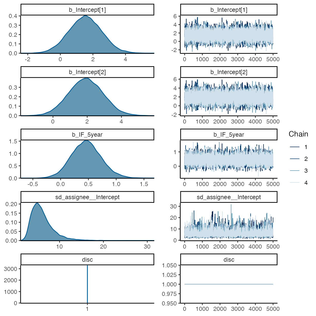
pp_check(m_h1, type = "bars", draws = 50)
#> Using 10 posterior draws for ppc type 'bars' by default.
#> Warning: The following arguments were unrecognized and ignored: draws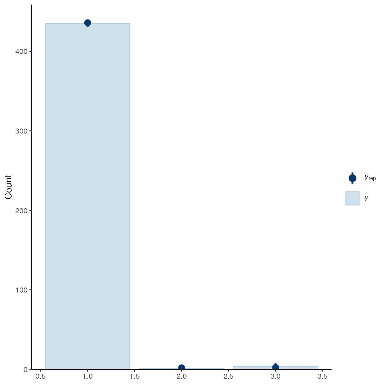
plot(equivalence_test(m_h1))
#> Picking joint bandwidth of 0.0295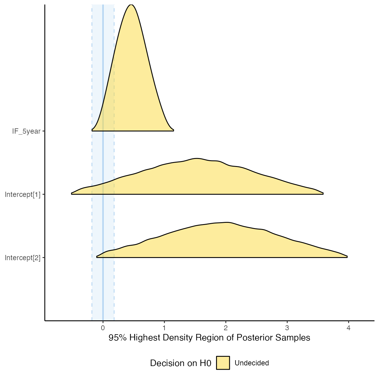
# pander(m_h1_report <- report(m_h1))
#
# m_h1_es <- report_effectsize(m_h1)
Data Availability
Test for any effects of the five year impact factor on the data’s availability.
rrpp <- import_notes()
rrpp <- drop_na(rrpp, data_avail)
m_h2 <-
brm(
formula = data_avail ~ IF_5year +
(1 | assignee),
data = rrpp,
seed = 27,
prior = priors,
family = cumulative(link = "logit"),
control = list(adapt_delta = 0.99),
iter = 10000,
chains = 4
)
#> Compiling Stan program...
#> Start sampling
summary(m_h2)
#> Family: cumulative
#> Links: mu = logit; disc = identity
#> Formula: data_avail ~ IF_5year + (1 | assignee)
#> Data: rrpp (Number of observations: 448)
#> Draws: 4 chains, each with iter = 10000; warmup = 5000; thin = 1;
#> total post-warmup draws = 20000
#>
#> Multilevel Hyperparameters:
#> ~assignee (Number of levels: 5)
#> Estimate Est.Error l-95% CI u-95% CI Rhat Bulk_ESS Tail_ESS
#> sd(Intercept) 2.15 1.29 0.33 5.26 1.00 2920 2559
#>
#> Regression Coefficients:
#> Estimate Est.Error l-95% CI u-95% CI Rhat Bulk_ESS Tail_ESS
#> Intercept[1] 0.85 0.67 -0.49 2.05 1.00 3789 5918
#> Intercept[2] 1.10 0.67 -0.24 2.29 1.00 3830 6128
#> Intercept[3] 1.53 0.67 0.19 2.73 1.00 3912 6177
#> IF_5year 0.15 0.08 -0.01 0.30 1.00 15775 12476
#>
#> Further Distributional Parameters:
#> Estimate Est.Error l-95% CI u-95% CI Rhat Bulk_ESS Tail_ESS
#> disc 1.00 0.00 1.00 1.00 NA NA NA
#>
#> Draws were sampled using sampling(NUTS). For each parameter, Bulk_ESS
#> and Tail_ESS are effective sample size measures, and Rhat is the potential
#> scale reduction factor on split chains (at convergence, Rhat = 1).
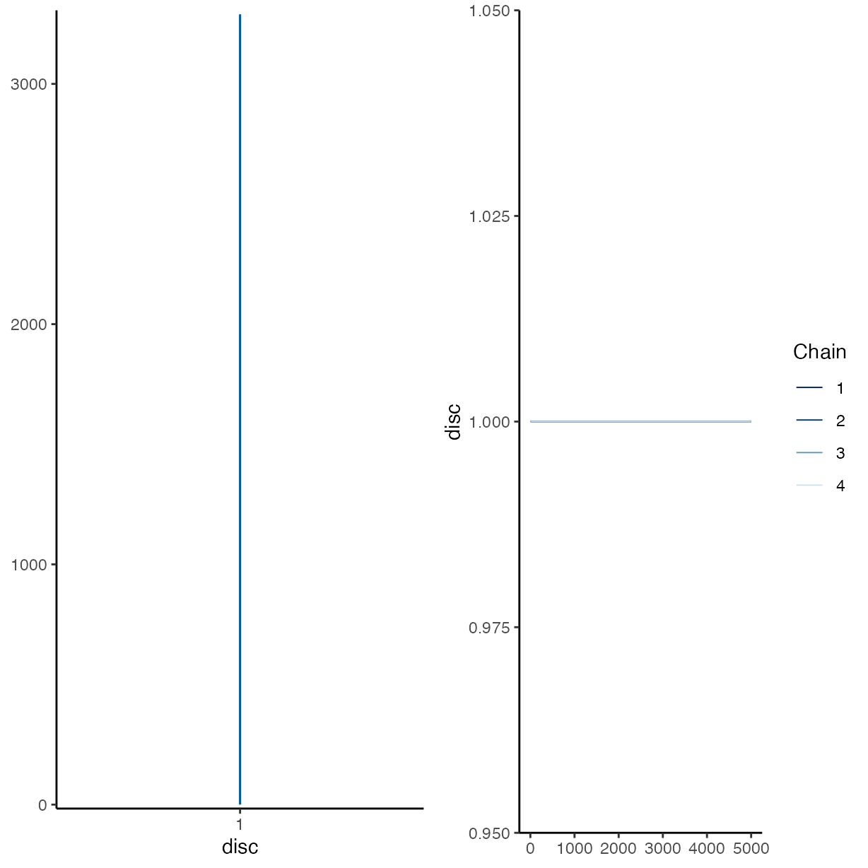
plot(m_h2)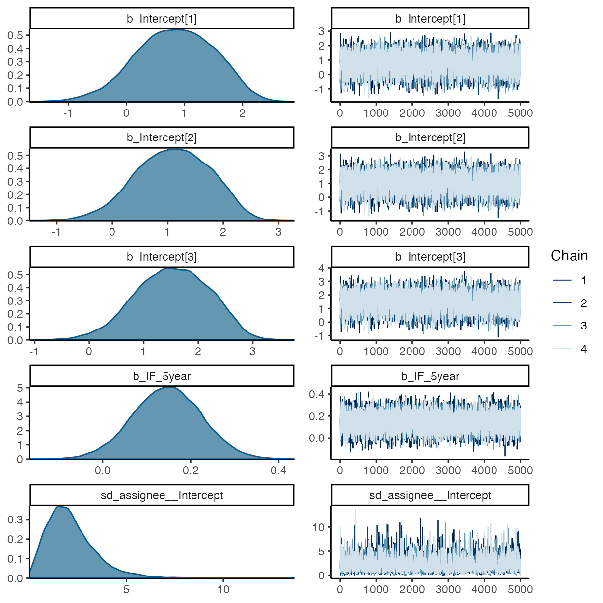
pp_check(m_h2, type = "bars", draws = 50)
#> Using 10 posterior draws for ppc type 'bars' by default.
#> Warning: The following arguments were unrecognized and ignored: draws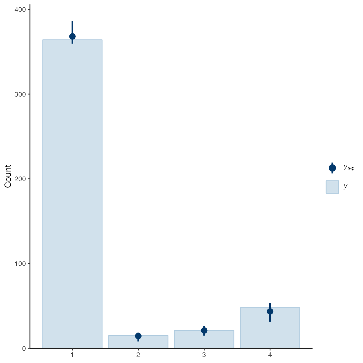
plot(equivalence_test(m_h2))
#> Picking joint bandwidth of 0.00866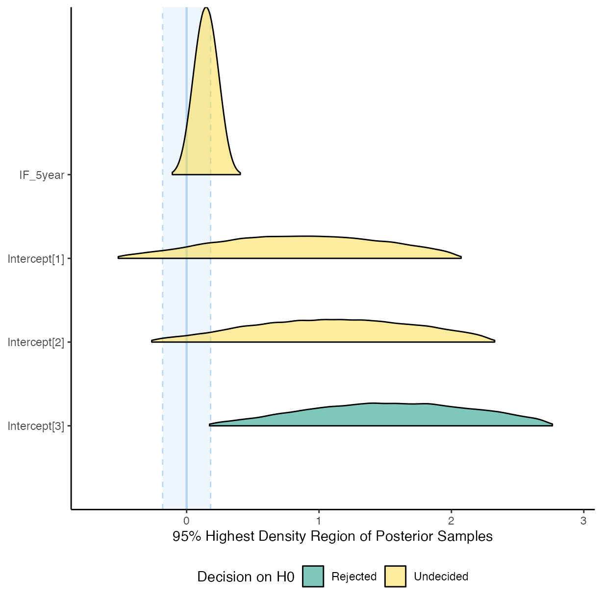
# pander(m_h2_report <- report(m_h2))
#
# m_h2_es <- report_effectsize(m_h2)
Save Model Objects
Save the model objects for figures in the paper.
save(m_h1, file = here("inst/extdata/m_h1.Rda"))
save(m_h2, file = here("inst/extdata/m_h2.Rda"))

save(m_h1_report, file = here("inst/extdata/m_h1_report.Rda"))
save(m_h2_report, file = here("inst/extdata/m_h2_report.Rda"))

save(m_h1_es, file = here("inst/extdata/m_h1_es.Rda"))
save(m_h2_es, file = here("inst/extdata/m_h2_es.Rda"))
Colophon
sessioninfo::session_info()
#> ─ Session info ───────────────────────────────────────────────────────────────
#>  setting  value
#>  version  R version 4.4.1 (2024-06-14)
#>  os       macOS Sonoma 14.6
#>  system   aarch64, darwin20
#>  ui       X11
#>  language en
#>  collate  en_US.UTF-8
#>  ctype    en_US.UTF-8
#>  tz       Australia/Perth
#>  date     2024-08-07
#>  pandoc   3.3 @ /opt/homebrew/bin/ (via rmarkdown)
#>
#> ─ Packages ───────────────────────────────────────────────────────────────────
#>  package                            * version  date (UTC) lib source
#>  abind                                1.4-5    2016-07-21 [1] CRAN (R 4.4.0)
#>  backports                            1.5.0    2024-05-23 [1] CRAN (R 4.4.0)
#>  bayesplot                          * 1.11.1   2024-02-15 [1] CRAN (R 4.4.0)
#>  bayestestR                         * 0.14.0   2024-07-24 [1] CRAN (R 4.4.0)
#>  bridgesampling                       1.1-2    2021-04-16 [1] CRAN (R 4.4.0)
#>  brms                               * 2.21.0   2024-03-20 [1] CRAN (R 4.4.1)
#>  Brobdingnag                          1.2-9    2022-10-19 [1] CRAN (R 4.4.0)
#>  bslib                                0.8.0    2024-07-29 [1] CRAN (R 4.4.0)
#>  cachem                               1.1.0    2024-05-16 [1] CRAN (R 4.4.0)
#>  callr                                3.7.6    2024-03-25 [1] CRAN (R 4.4.0)
#>  cellranger                           1.1.0    2016-07-27 [1] CRAN (R 4.4.0)
#>  checkmate                            2.3.2    2024-07-29 [1] CRAN (R 4.4.0)
#>  cli                                  3.6.3    2024-06-21 [1] CRAN (R 4.4.0)
#>  coda                                 0.19-4.1 2024-01-31 [1] CRAN (R 4.4.0)
#>  codetools                            0.2-20   2024-03-31 [2] CRAN (R 4.4.1)
#>  colorspace                           2.1-1    2024-07-26 [1] CRAN (R 4.4.0)
#>  curl                                 5.2.1    2024-03-01 [1] CRAN (R 4.4.0)
#>  datawizard                           0.12.2   2024-07-21 [1] CRAN (R 4.4.0)
#>  desc                                 1.4.3    2023-12-10 [1] CRAN (R 4.4.0)
#>  digest                               0.6.36   2024-06-23 [1] CRAN (R 4.4.0)
#>  distributional                       0.4.0    2024-02-07 [1] CRAN (R 4.4.0)
#>  dplyr                                1.1.4    2023-11-17 [1] CRAN (R 4.4.0)
#>  emmeans                              1.10.3   2024-07-01 [1] CRAN (R 4.4.0)
#>  estimability                         1.5.1    2024-05-12 [1] CRAN (R 4.4.0)
#>  evaluate                             0.24.0   2024-06-10 [1] CRAN (R 4.4.0)
#>  fansi                                1.0.6    2023-12-08 [1] CRAN (R 4.4.0)
#>  farver                               2.1.2    2024-05-13 [1] CRAN (R 4.4.0)
#>  fastmap                              1.2.0    2024-05-15 [1] CRAN (R 4.4.0)
#>  fs                                   1.6.4    2024-04-25 [1] CRAN (R 4.4.0)
#>  generics                             0.1.3    2022-07-05 [1] CRAN (R 4.4.0)
#>  ggplot2                            * 3.5.1    2024-04-23 [1] CRAN (R 4.4.0)
#>  ggridges                             0.5.6    2024-01-23 [1] CRAN (R 4.4.0)
#>  glue                                 1.7.0    2024-01-09 [1] CRAN (R 4.4.0)
#>  gridExtra                            2.3      2017-09-09 [1] CRAN (R 4.4.0)
#>  gtable                               0.3.5    2024-04-22 [1] CRAN (R 4.4.0)
#>  here                               * 1.0.1    2020-12-13 [1] CRAN (R 4.4.0)
#>  highr                                0.11     2024-05-26 [1] CRAN (R 4.4.0)
#>  htmltools                            0.5.8.1  2024-04-04 [1] CRAN (R 4.4.0)
#>  htmlwidgets                          1.6.4    2023-12-06 [1] CRAN (R 4.4.0)
#>  inline                               0.3.19   2021-05-31 [1] CRAN (R 4.4.0)
#>  insight                              0.20.2   2024-07-13 [1] CRAN (R 4.4.0)
#>  jquerylib                            0.1.4    2021-04-26 [1] CRAN (R 4.4.0)
#>  jsonlite                             1.8.8    2023-12-04 [1] CRAN (R 4.4.0)
#>  knitr                                1.48     2024-07-07 [1] CRAN (R 4.4.0)
#>  labeling                             0.4.3    2023-08-29 [1] CRAN (R 4.4.0)
#>  lattice                              0.22-6   2024-03-20 [2] CRAN (R 4.4.1)
#>  lifecycle                            1.0.4    2023-11-07 [1] CRAN (R 4.4.0)
#>  loo                                  2.8.0    2024-07-03 [1] CRAN (R 4.4.0)
#>  magrittr                             2.0.3    2022-03-30 [1] CRAN (R 4.4.0)
#>  MASS                                 7.3-60.2 2024-04-26 [2] CRAN (R 4.4.1)
#>  Matrix                               1.7-0    2024-04-26 [2] CRAN (R 4.4.1)
#>  matrixStats                          1.3.0    2024-04-11 [1] CRAN (R 4.4.0)
#>  minty                                0.0.1    2024-05-22 [1] CRAN (R 4.4.0)
#>  multcomp                             1.4-26   2024-07-18 [1] CRAN (R 4.4.0)
#>  munsell                              0.5.1    2024-04-01 [1] CRAN (R 4.4.0)
#>  mvtnorm                              1.2-5    2024-05-21 [1] CRAN (R 4.4.0)
#>  nlme                                 3.1-164  2023-11-27 [2] CRAN (R 4.4.1)
#>  pander                             * 0.6.5    2022-03-18 [1] CRAN (R 4.4.0)
#>  pillar                               1.9.0    2023-03-22 [1] CRAN (R 4.4.0)
#>  pkgbuild                             1.4.4    2024-03-17 [1] CRAN (R 4.4.0)
#>  pkgconfig                            2.0.3    2019-09-22 [1] CRAN (R 4.4.0)
#>  pkgdown                              2.1.0    2024-07-06 [1] CRAN (R 4.4.0)
#>  plyr                                 1.8.9    2023-10-02 [1] CRAN (R 4.4.0)
#>  posterior                            1.6.0    2024-07-03 [1] CRAN (R 4.4.0)
#>  processx                             3.8.4    2024-03-16 [1] CRAN (R 4.4.0)
#>  ps                                   1.7.7    2024-07-02 [1] CRAN (R 4.4.0)
#>  purrr                                1.0.2    2023-08-10 [1] CRAN (R 4.4.0)
#>  QuickJSR                             1.3.1    2024-07-14 [1] CRAN (R 4.4.0)
#>  R6                                   2.5.1    2021-08-19 [1] CRAN (R 4.4.0)
#>  ragg                                 1.3.2    2024-05-15 [1] CRAN (R 4.4.0)
#>  Rcpp                               * 1.0.13   2024-07-17 [1] CRAN (R 4.4.0)
#>  RcppParallel                         5.1.8    2024-07-06 [1] CRAN (R 4.4.0)
#>  readODS                              2.3.0    2024-05-26 [1] CRAN (R 4.4.0)
#>  report                             * 0.4.0    2021-09-30 [1] CRAN (R 4.4.1)
#>  Reproducibility.in.Plant.Pathology * 1.0.2    2024-08-06 [1] Github (openplantpathology/Reproducibility_in_Plant_Pathology@240170e)
#>  reshape2                             1.4.4    2020-04-09 [1] CRAN (R 4.4.0)
#>  rlang                                1.1.4    2024-06-04 [1] CRAN (R 4.4.0)
#>  rmarkdown                            2.27     2024-05-17 [1] CRAN (R 4.4.0)
#>  rprojroot                            2.0.4    2023-11-05 [1] CRAN (R 4.4.0)
#>  rstan                                2.32.6   2024-03-05 [1] CRAN (R 4.4.1)
#>  rstantools                           2.4.0    2024-01-31 [1] CRAN (R 4.4.0)
#>  rstudioapi                           0.16.0   2024-03-24 [1] CRAN (R 4.4.0)
#>  sandwich                             3.1-0    2023-12-11 [1] CRAN (R 4.4.0)
#>  sass                                 0.4.9    2024-03-15 [1] CRAN (R 4.4.0)
#>  scales                               1.3.0    2023-11-28 [1] CRAN (R 4.4.0)
#>  see                                  0.8.5    2024-07-17 [1] CRAN (R 4.4.0)
#>  sessioninfo                          1.2.2    2021-12-06 [1] CRAN (R 4.4.0)
#>  StanHeaders                          2.32.10  2024-07-15 [1] CRAN (R 4.4.0)
#>  stringi                              1.8.4    2024-05-06 [1] CRAN (R 4.4.0)
#>  stringr                              1.5.1    2023-11-14 [1] CRAN (R 4.4.0)
#>  survival                             3.6-4    2024-04-24 [2] CRAN (R 4.4.1)
#>  systemfonts                          1.1.0    2024-05-15 [1] CRAN (R 4.4.0)
#>  tensorA                              0.36.2.1 2023-12-13 [1] CRAN (R 4.4.0)
#>  textshaping                          0.4.0    2024-05-24 [1] CRAN (R 4.4.0)
#>  TH.data                              1.1-2    2023-04-17 [1] CRAN (R 4.4.0)
#>  tibble                               3.2.1    2023-03-20 [1] CRAN (R 4.4.0)
#>  tidyr                              * 1.3.1    2024-01-24 [1] CRAN (R 4.4.0)
#>  tidyselect                           1.2.1    2024-03-11 [1] CRAN (R 4.4.0)
#>  tzdb                                 0.4.0    2023-05-12 [1] CRAN (R 4.4.0)
#>  utf8                                 1.2.4    2023-10-22 [1] CRAN (R 4.4.0)
#>  V8                                   4.4.2    2024-02-15 [1] CRAN (R 4.4.0)
#>  vctrs                                0.6.5    2023-12-01 [1] CRAN (R 4.4.0)
#>  withr                                3.0.1    2024-07-31 [1] CRAN (R 4.4.0)
#>  xfun                                 0.46     2024-07-18 [1] CRAN (R 4.4.0)
#>  xtable                               1.8-4    2019-04-21 [1] CRAN (R 4.4.0)
#>  yaml                                 2.3.10   2024-07-26 [1] CRAN (R 4.4.0)
#>  zip                                  2.3.1    2024-01-27 [1] CRAN (R 4.4.0)
#>  zoo                                  1.8-12   2023-04-13 [1] CRAN (R 4.4.0)
#>
#>  [1] /Users/283204f/Library/R/arm64/4.4/library
#>  [2] /Library/Frameworks/R.framework/Versions/4.4-arm64/Resources/library
#>
#> ──────────────────────────────────────────────────────────────────────────────