Data Visualisation

This vignette documents a simple visualisation and tabulation of the data gathered from surveying 21 journals and 450 articles in the field of plant pathology for their openness and reproducibility.

Set-up Workspace

Load libraries used and setting the ggplot2 theme for the document.

library("tidyverse")
#> ── Attaching packages ─────────────────────────────────────── tidyverse 1.3.2 ──
#> ✔ ggplot2 3.4.0      ✔ purrr   1.0.0 
#> ✔ tibble  3.1.8      ✔ dplyr   1.0.10
#> ✔ tidyr   1.2.1      ✔ stringr 1.5.0 
#> ✔ readr   2.1.3      ✔ forcats 0.5.2 
#> ── Conflicts ────────────────────────────────────────── tidyverse_conflicts() ──
#> ✖ dplyr::filter() masks stats::filter()
#> ✖ dplyr::lag()    masks stats::lag()
library("janitor")
#> 
#> Attaching package: 'janitor'
#> 
#> The following objects are masked from 'package:stats':
#> 
#>     chisq.test, fisher.test
library("pander")
library("Reproducibility.in.Plant.Pathology")
theme_set(theme_classic())

Import the data and calculate the reproducibility score

rrpp <- import_notes()

Individual Rating Scores

rrpp %>%
  mutate(
    comp_mthds_avail = as.numeric(as.character(comp_mthds_avail)),
    data_avail =  as.numeric(as.character(data_avail))
  ) %>%
  pivot_longer(cols = c("comp_mthds_avail",
                        "data_avail")) %>%
  ggplot(aes(x = as.factor(value))) +
  geom_bar() +
  ylab("Count") +
  xlab("Criteria Score") +
  ggtitle("Criteria scores by evaluator") +
  facet_grid(name ~ assignee)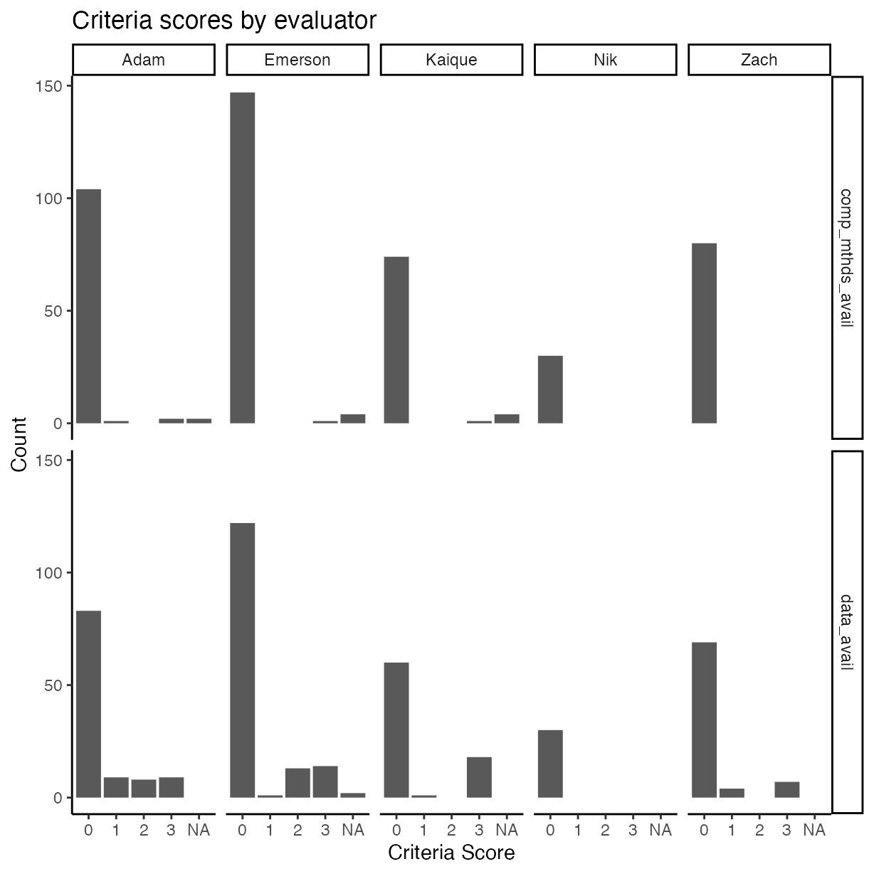

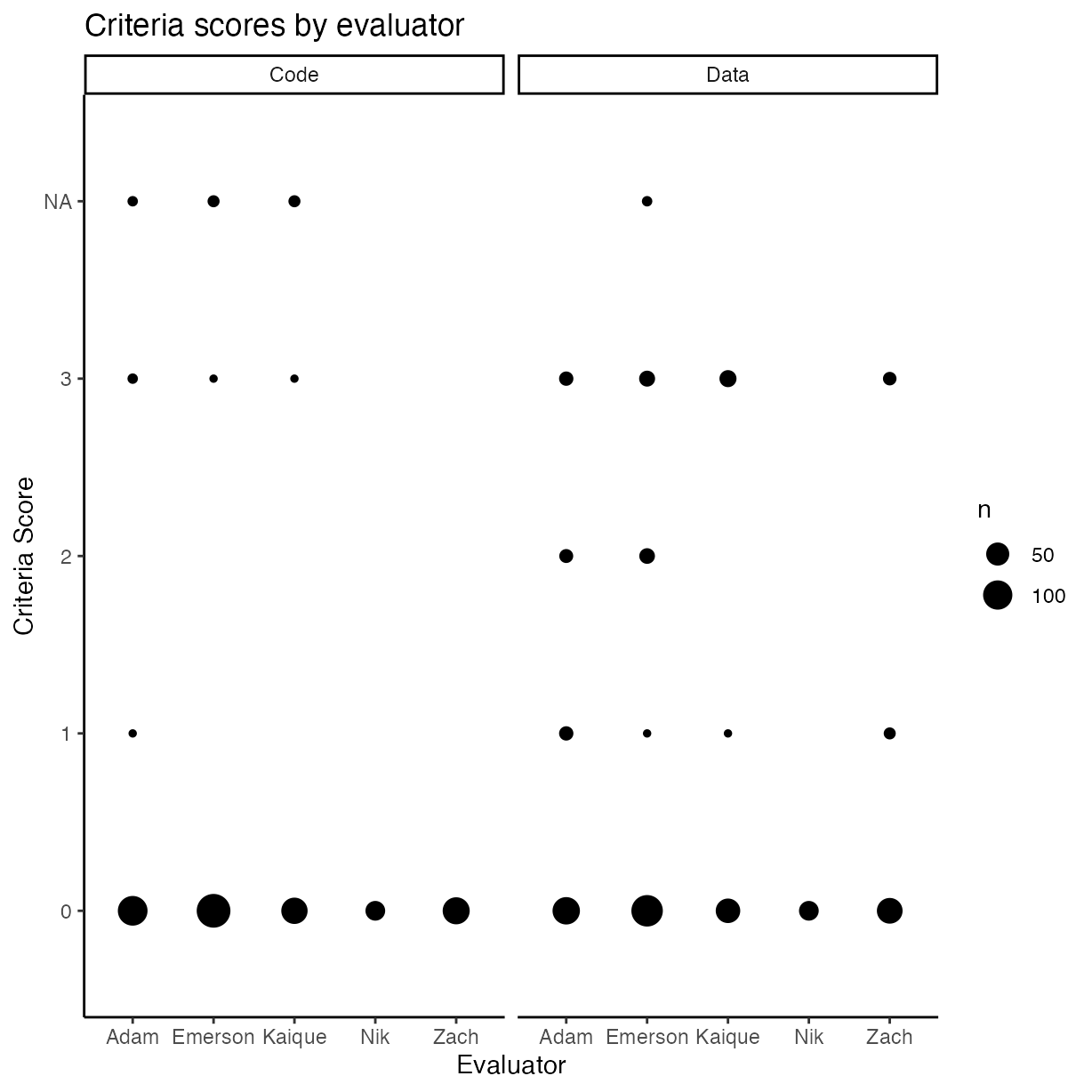
rrpp %>%
  mutate(
    comp_mthds_avail = as.numeric(as.character(comp_mthds_avail)),
    data_avail =  as.numeric(as.character(data_avail))
  ) %>%
  pivot_longer(cols = c("comp_mthds_avail",
                        "data_avail")) %>%
  ggplot(aes(y = as.factor(value), x = assignee)) +
  geom_count() +
  ylab("Criteria Score") +
  xlab("Evaluator") +
  ggtitle("Criteria scores by evaluator") +
  facet_wrap(name ~ .,
             labeller = labeller(name =
                                   c(
                                     "comp_mthds_avail" = "Code",
                                     "data_avail" = "Data"
                                   )))

Visualise evaluations

Computational methods available

Were the computational methods, scripts, source code, etc., made available?

ggplot(rrpp, aes(y = as.factor(comp_mthds_avail))) +
  geom_bar() +
  ggtitle("Computational Methods Availability") +
  ylab("Score") +
  labs(caption = "NA means that no computational methods were used to generate the data,\ne.g. only PCR results reported with no statistical analysis")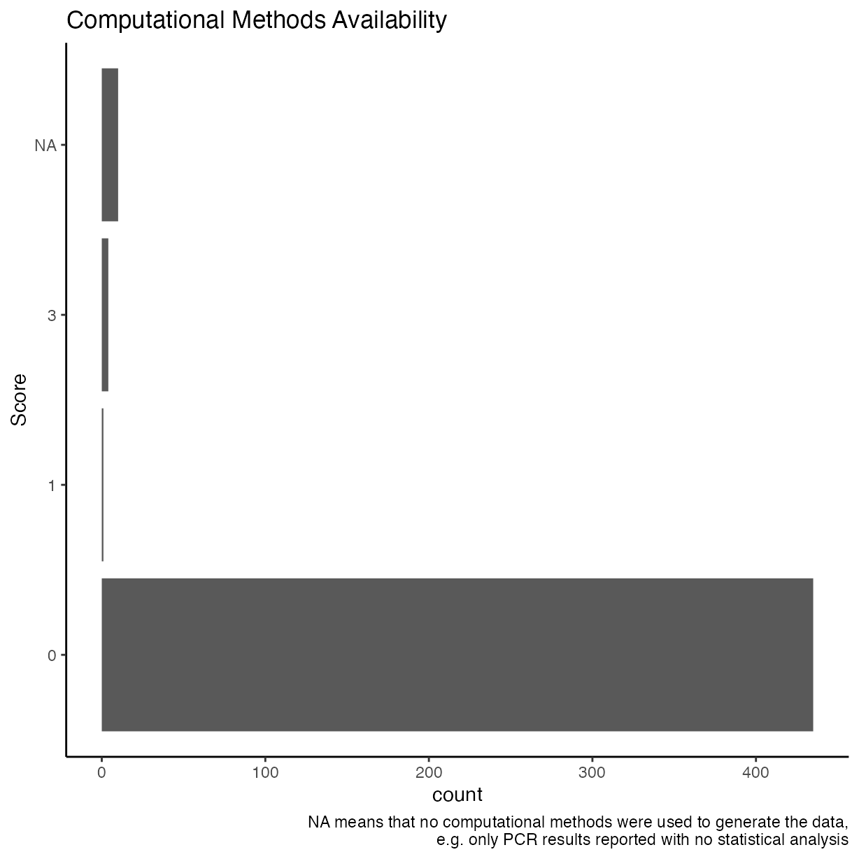

Software used (cited)

Count and sort top 10 software packages cited. There are likely others that are used, but they have not been properly cited or listed by the authors.

First create a tidy data frame of the data by unnesting software used as in many cases multiple software packages were used, so will end up with multiple rows for same article, one for each software.

rrpp_software <-
  rrpp %>%
  transform(software_used = strsplit(software_used, ",")) %>%
  unnest(software_used) %>%
  mutate(software_used = trimws(software_used)) %>%
  mutate(software_used = toupper(software_used)) # convert all to uppercase to standardise

Now graph the top ten software packages used.

tab <- table(rrpp_software$software_used)
tab_s <- as.data.frame(sort(tab))
tab_s <-
  tab_s %>%
  arrange(desc(Freq)) %>%
  filter(Freq %in% head(unique(Freq), 10)) %>% 
  rename("Software" = "Var1", "Frequency" = "Freq")

ggplot(tab_s, aes(y = Software, x = Frequency)) +
  geom_bar(stat = "identity") +
  ggtitle("Top 10 Software Used") +
  xlab("Count") +
  ylab("Software")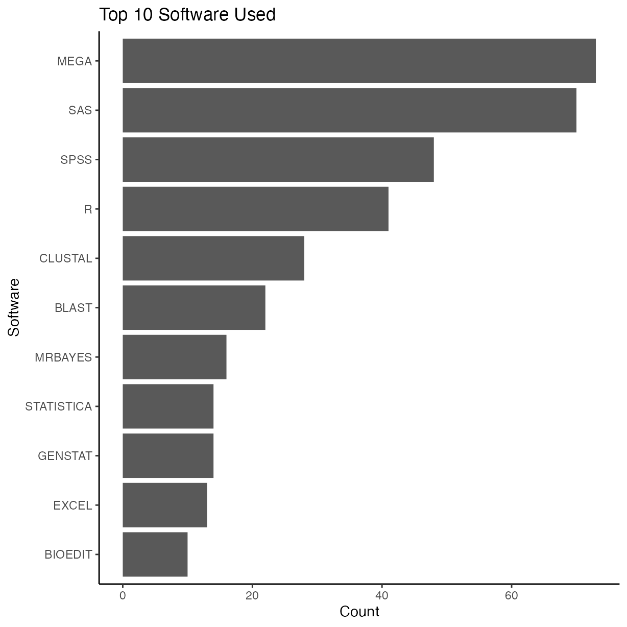

Data availability

Were the data made readily available?

ggplot(rrpp, aes(y = as.factor(data_avail))) +
  geom_bar() +
  ggtitle("Data Availability") +
  ylab("Score")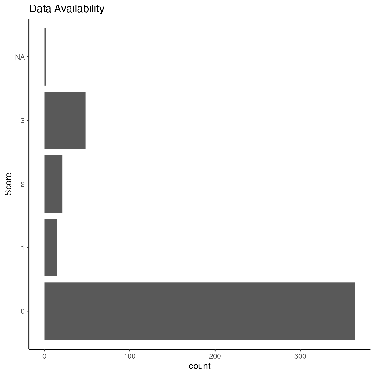

Scores by year

rrpp %>%
  pivot_longer(cols = c("comp_mthds_avail", "data_avail")) %>%
  ggplot(aes(x = year,
             y = value)) +
  geom_count() +
  ylab("Score") +
  xlab("Year") +
  facet_grid(name ~ .)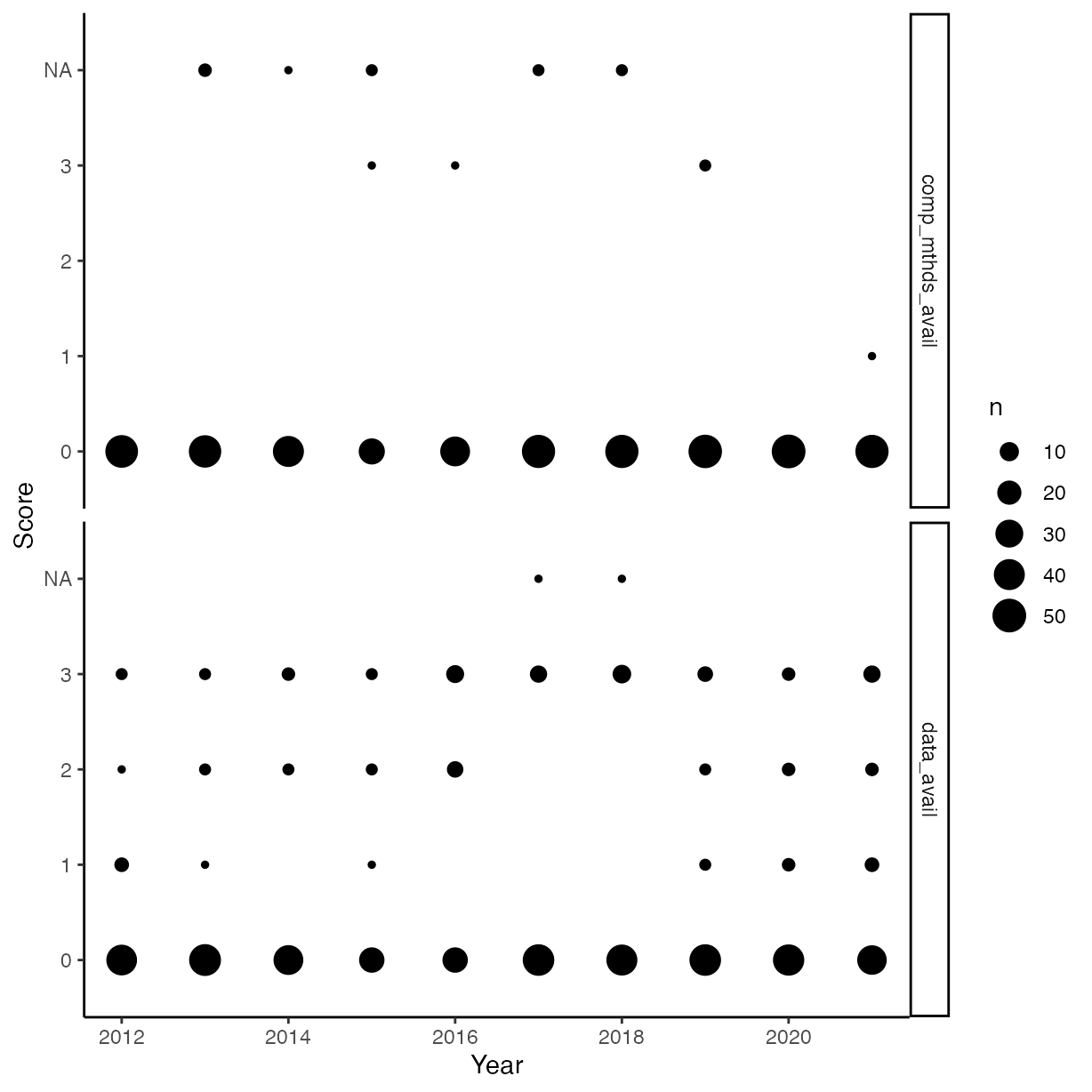

Visualise Probabilities

Code Availability

rrpp %>%
  group_by(comp_mthds_avail) %>%
  drop_na(comp_mthds_avail) %>%
  count() %>%
  mutate(pr_k = n / nrow(drop_na(rrpp, comp_mthds_avail))) %>%
  ungroup() %>%
  mutate(cum_pr_k = cumsum(pr_k)) %>% 
  
  ggplot(aes(x = as.numeric(as.character(comp_mthds_avail)), y = cum_pr_k, 
             fill = as.numeric(as.character(comp_mthds_avail)))) +
  geom_line() +
  geom_point(shape = 21,
             colour = "grey92", 
             size = 2.5,
             stroke = 1) +
  scale_y_continuous("cumulative proportion", breaks = c(0, .5, 1)) +
  scale_fill_gradient() +
  coord_cartesian(ylim = c(0, 1)) +
  theme(legend.position = "none") +
  xlab("Computational Methods Availability Score")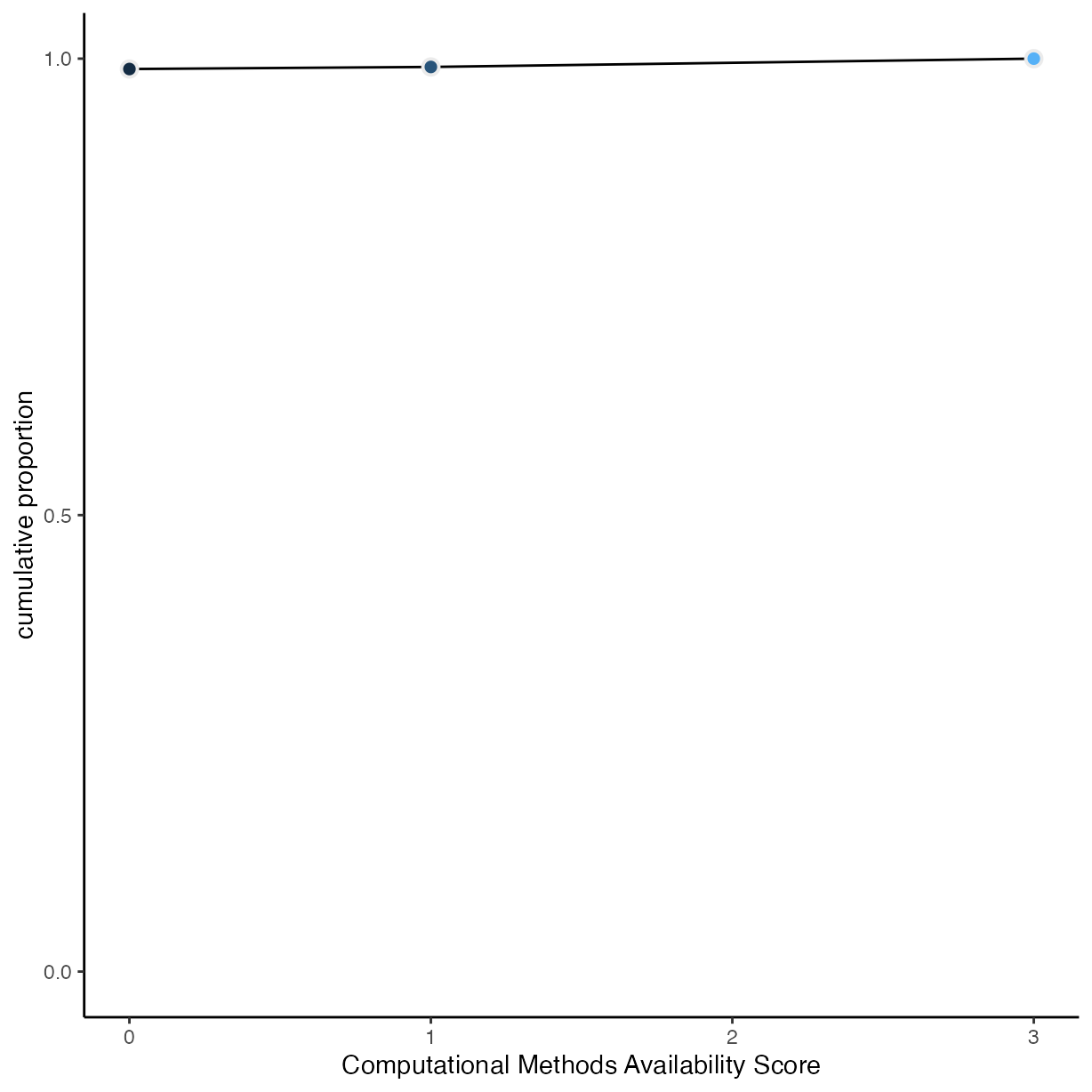

# McElreath's convenience function from page 335
logit <- function(x) log(x / (1 - x))

rrpp %>%
  group_by(comp_mthds_avail) %>%
  drop_na(comp_mthds_avail) %>%
  count() %>%
  mutate(pr_k = n / nrow(drop_na(rrpp, comp_mthds_avail))) %>%
  ungroup() %>%
  mutate(cum_pr_k = cumsum(pr_k)) %>%
  filter(comp_mthds_avail < 3) %>%
  ggplot(aes(
    x = as.numeric(as.character(comp_mthds_avail)),
    y = logit(cum_pr_k),
    fill = as.numeric(as.character(comp_mthds_avail))
  )) +
  geom_line() +
  geom_point(
    shape = 21,
    colour = "grey92",
    size = 2.5,
    stroke = 1
  ) +
  coord_cartesian(xlim = c(0, 3)) +
  ylab("log-cumulative-odds") +
  xlab("Code Availability") +
  scale_fill_gradient() +
  theme(legend.position = "none")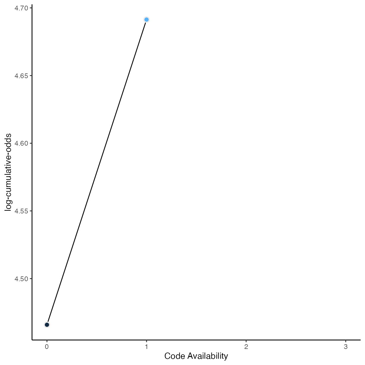

Data Availability

rrpp %>%
  group_by(data_avail) %>%
  drop_na(data_avail) %>%
  count() %>%
  mutate(pr_k = n / nrow(drop_na(rrpp, data_avail))) %>%
  ungroup() %>%
  mutate(cum_pr_k = cumsum(pr_k)) %>% 
  ggplot(aes(x = as.numeric(as.character(data_avail)), y = cum_pr_k, 
             fill = as.numeric(as.character(data_avail)))) +
  geom_line() +
  geom_point(shape = 21,
             colour = "grey92", 
             size = 2.5,
             stroke = 1) +
  scale_y_continuous("cumulative proportion", breaks = c(0, .5, 1)) +
  scale_fill_gradient() +
  coord_cartesian(ylim = c(0, 1)) +
  theme(legend.position = "none") +
  xlab("Data Availability Score")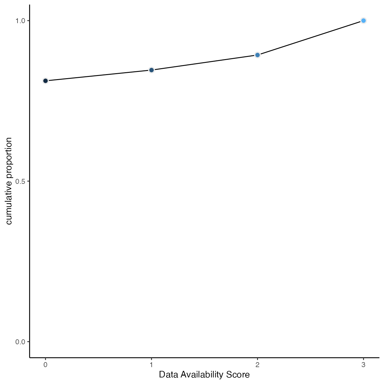

rrpp %>%
  group_by(data_avail) %>%
  drop_na(data_avail) %>%
  count() %>%
  mutate(pr_k = n / nrow(drop_na(rrpp, data_avail))) %>%
  ungroup() %>%
  mutate(cum_pr_k = cumsum(pr_k)) %>%
  filter(data_avail < 3) %>%
  ggplot(aes(
    x = as.numeric(as.character(data_avail)),
    y = logit(cum_pr_k),
    fill = as.numeric(as.character(data_avail))
  )) +
  geom_line() +
  geom_point(
    shape = 21,
    colour = "grey92",
    size = 2.5,
    stroke = 1
  ) +
  coord_cartesian(xlim = c(0, 3)) +
  ylab("log-cumulative-odds") +
  xlab("Code Availability") +
  scale_fill_gradient() +
  theme(legend.position = "none")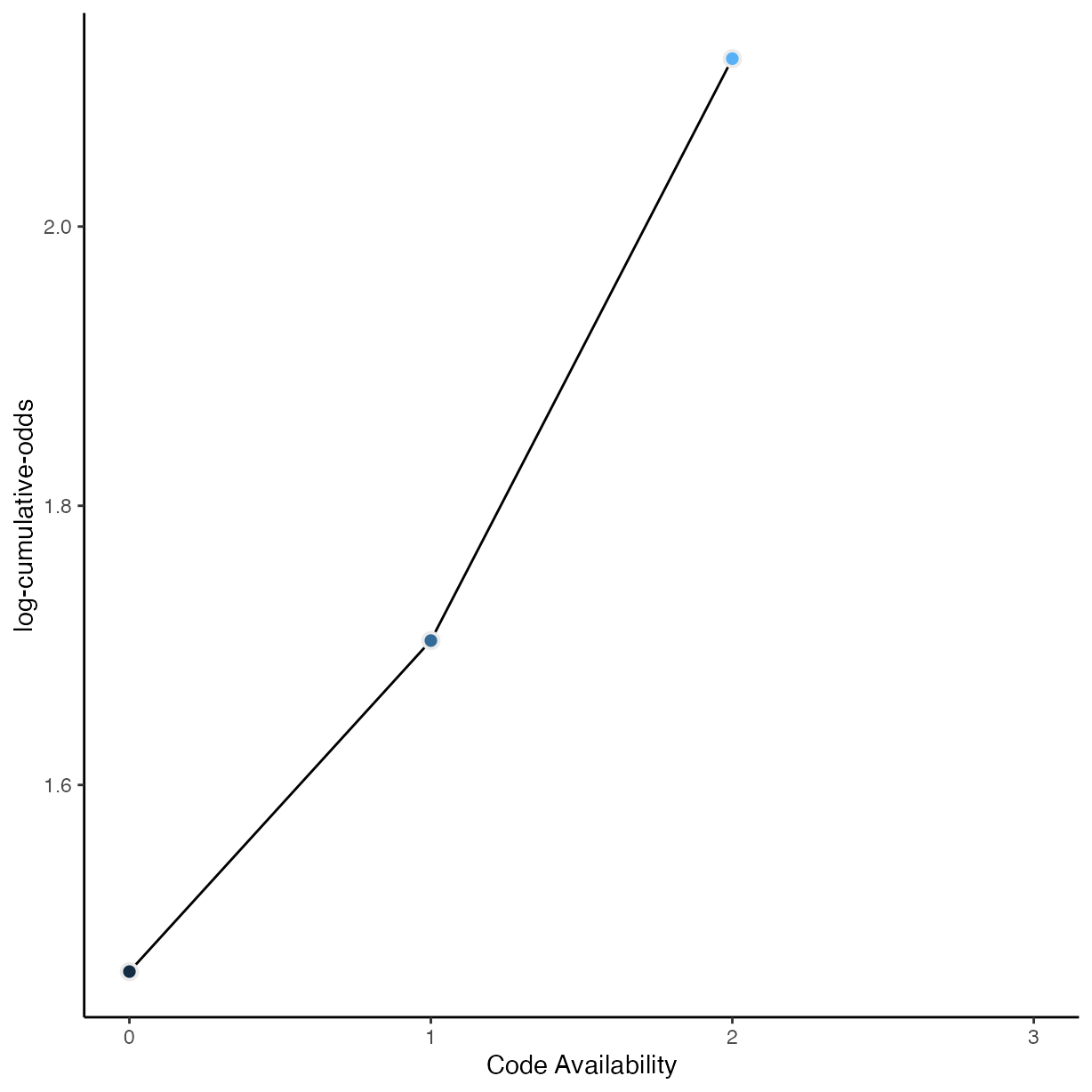

Tables

Table of journals surveyed

rrpp_journals <- tabyl(rrpp, journal)[, -3]
names(rrpp_journals) <- c("Journal", "n")
pander(rrpp_journals)

Journal	n
Australasian Plant Pathology	11
Canadian Journal of Plant Pathology	19
Crop Protection	23
European Journal of Plant Pathology	19
Forest Pathology	18
Journal of General Plant Pathology	24
Journal of Phytopathology	19
Journal of Plant Pathology	23
Molecular Plant Pathology	29
Molecular Plant-Microbe Interactions	22
Nematology	16
Physiological and Molecular Plant Pathology	24
Phytoparasitica	23
Phytopathologia Mediterranea	20
Phytopathology	28
Plant Disease	24
Plant Health Progress	16
Plant Pathology	30
Revista Mexicana de Fitopatología	19
Tropical Plant Pathology	18
Virology Journal (Plant Viruses Section)	25

Adam H. Sparks

2023-01-04