Analysis of Publication Year Effect

This vignette documents the analysis of the data gathered from surveying 21 journals and 450 articles in the field of plant pathology for their openness and reproducibility and the effect that the publication year had on that score.

Set-up Workspace

Load libraries used and setting the ggplot2 theme for the document.

library("brms")
library("bayestestR")
library("bayesplot")
library("ggplot2")
library("here")
library("pander")
library("report")
library("tidyr")
library("Reproducibility.in.Plant.Pathology")

options(mc.cores = parallel::detectCores())
theme_set(theme_classic())

Priors

Priors were set to be generic weakly informative.

priors <- c(prior(normal(0, 1), class = "b"),
            prior(normal(0, 1), class = "Intercept"))

Year of Publication Effect Models

Computational Methods Availability

Test the effect that year of publication had on the code availability and detect differences over time. Here, year is a fixed effect, journal and assignee are assigned as random effects.

rrpp <- import_notes()
rrpp <- drop_na(rrpp, comp_mthds_avail)

m_g1 <-
  brm(
    formula = comp_mthds_avail ~ year +
      (1 | abbreviation) +
      (1 | assignee),
    data = rrpp,
    seed = 27,
    prior = priors,
    family = cumulative(link = "logit"),
    iter = 10000,
    control = list(adapt_delta = 0.9999),
  )
#> Compiling Stan program...
#> Start sampling

summary(m_g1)
#>  Family: cumulative 
#>   Links: mu = logit; disc = identity 
#> Formula: comp_mthds_avail ~ year + (1 | abbreviation) + (1 | assignee) 
#>    Data: rrpp (Number of observations: 440) 
#>   Draws: 4 chains, each with iter = 10000; warmup = 5000; thin = 1;
#>          total post-warmup draws = 20000
#> 
#> Group-Level Effects: 
#> ~abbreviation (Number of levels: 20) 
#>               Estimate Est.Error l-95% CI u-95% CI Rhat Bulk_ESS Tail_ESS
#> sd(Intercept)     1.52      0.94     0.12     3.74 1.00     6752     6340
#> 
#> ~assignee (Number of levels: 5) 
#>               Estimate Est.Error l-95% CI u-95% CI Rhat Bulk_ESS Tail_ESS
#> sd(Intercept)     7.12      3.24     3.08    15.15 1.00     6731    10385
#> 
#> Population-Level Effects: 
#>              Estimate Est.Error l-95% CI u-95% CI Rhat Bulk_ESS Tail_ESS
#> Intercept[1]   406.87    354.02  -259.06  1135.27 1.00    19328    13013
#> Intercept[2]   407.27    354.03  -258.92  1135.69 1.00    19328    13013
#> year             0.20      0.18    -0.13     0.56 1.00    19316    13013
#> 
#> Family Specific Parameters: 
#>      Estimate Est.Error l-95% CI u-95% CI Rhat Bulk_ESS Tail_ESS
#> disc     1.00      0.00     1.00     1.00   NA       NA       NA
#> 
#> Draws were sampled using sampling(NUTS). For each parameter, Bulk_ESS
#> and Tail_ESS are effective sample size measures, and Rhat is the potential
#> scale reduction factor on split chains (at convergence, Rhat = 1).

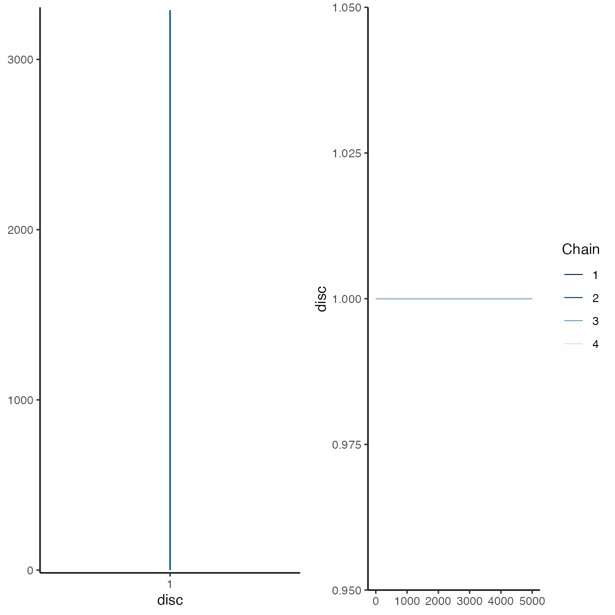
plot(m_g1)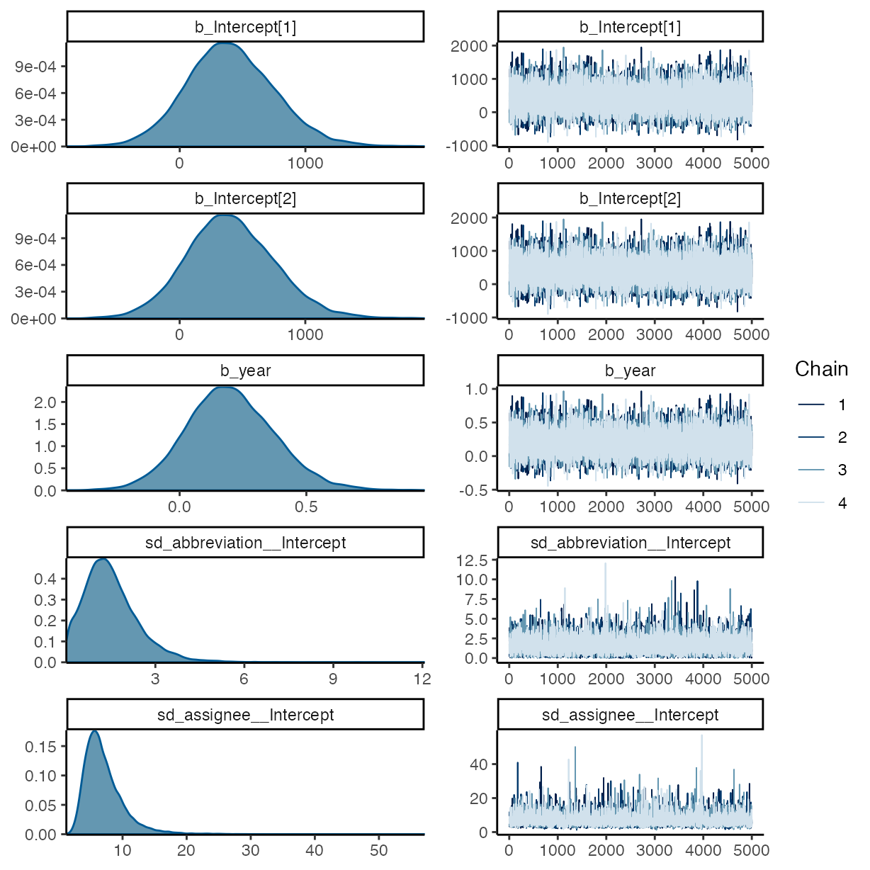


pp_check(m_g1, ndraws = 50, type = "bars")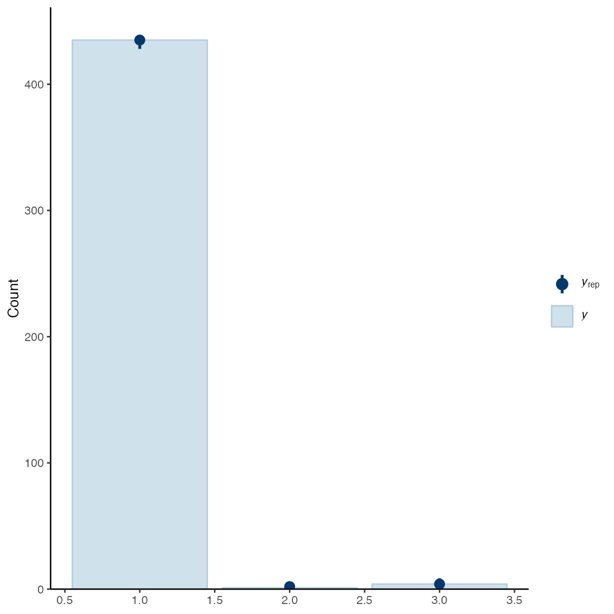


plot(equivalence_test(m_g1))
#> Picking joint bandwidth of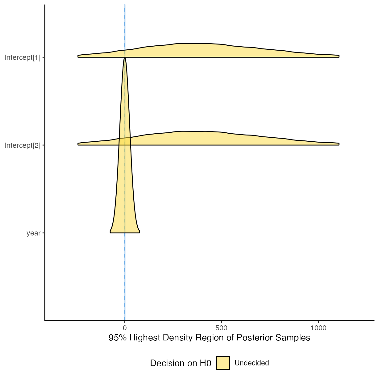 25.4
#> Warning: Removed 3000 rows containing non-finite values
#> (`stat_density_ridges()`).


pander(m_g1_report <- report(m_g1))
#> Warning: Predictions are treated as continuous variables in 'bayes_R2' which is
#> likely invalid for ordinal families.
#> Warning: Predictions are treated as continuous variables in 'bayes_R2' which is
#> likely invalid for ordinal families.
#> Start sampling
#> Warning: Predictions are treated as continuous variables in 'bayes_R2' which is
#> likely invalid for ordinal families.

#> Warning: Predictions are treated as continuous variables in 'bayes_R2' which is
#> likely invalid for ordinal families.

_We fitted a Bayesian logistic mixed model (estimated using MCMC sampling with 4 chains of 10000 iterations and a warmup of 5000) to predict comp_mthds_avail with year (formula: comp_mthds_avail ~ year). The model included abbreviation as random effects (formula: list(~1 | abbreviation, ~1 | assignee)). Priors over parameters were set as normal (mean = 0.00, SD = 1.00) distributions. The model’s explanatory power is weak (R2 = 0.06, 95% CI [4.71e-04, 0.24]) and the part related to the fixed effects alone (marginal R2) is of 0.38 (95% CI [0.01, 0.48]). Within this model:

The effect of b Intercept[1] (Median = 393.30, 95% CI [-259.06, 1135.27]) has a 88.33% probability of being positive (> 0), 88.33% of being significant (> 0.05), and 88.28% of being large (> 0.30). The estimation successfully converged (Rhat = 1.000) and the indices are reliable (ESS = 18761)
The effect of b Intercept[2] (Median = 393.71, 95% CI [-258.92, 1135.69]) has a 88.35% probability of being positive (> 0), 88.35% of being significant (> 0.05), and 88.33% of being large (> 0.30). The estimation successfully converged (Rhat = 1.000) and the indices are reliable (ESS = 18760)
The effect of b year (Median = 0.19, 95% CI [-0.13, 0.56]) has a 88.30% probability of being positive (> 0), 81.12% of being significant (> 0.05), and 27.50% of being large (> 0.30). The estimation successfully converged (Rhat = 1.000) and the indices are reliable (ESS = 18749)

Following the Sequential Effect eXistence and sIgnificance Testing (SEXIT) framework, we report the median of the posterior distribution and its 95% CI (Highest Density Interval), along the probability of direction (pd), the probability of significance and the probability of being large. The thresholds beyond which the effect is considered as significant (i.e., non-negligible) and large are |0.05| and |0.30|. Convergence and stability of the Bayesian sampling has been assessed using R-hat, which should be below 1.01 (Vehtari et al., 2019), and Effective Sample Size (ESS), which should be greater than 1000 (Burkner, 2017)._, _We fitted a Bayesian logistic mixed model (estimated using MCMC sampling with 4 chains of 10000 iterations and a warmup of 5000) to predict comp_mthds_avail with year (formula: comp_mthds_avail ~ year). The model included abbreviation as random effects (formula: list(~1 | abbreviation, ~1 | assignee)). Priors over parameters were set as normal (mean = 0.00, SD = 1.00) distributions. The model’s explanatory power is weak (R2 = 0.06, 95% CI [4.71e-04, 0.24]) and the part related to the fixed effects alone (marginal R2) is of 0.38 (95% CI [0.01, 0.48]). Within this model:

The effect of b Intercept[1] (Median = 393.30, 95% CI [-259.06, 1135.27]) has a 88.33% probability of being positive (> 0), 88.33% of being significant (> 0.05), and 88.28% of being large (> 0.30). The estimation successfully converged (Rhat = 1.000) and the indices are reliable (ESS = 18761)
The effect of b Intercept[2] (Median = 393.71, 95% CI [-258.92, 1135.69]) has a 88.35% probability of being positive (> 0), 88.35% of being significant (> 0.05), and 88.33% of being large (> 0.30). The estimation successfully converged (Rhat = 1.000) and the indices are reliable (ESS = 18760)
The effect of b year (Median = 0.19, 95% CI [-0.13, 0.56]) has a 88.30% probability of being positive (> 0), 81.12% of being significant (> 0.05), and 27.50% of being large (> 0.30). The estimation successfully converged (Rhat = 1.000) and the indices are reliable (ESS = 18749)

The effect of b Intercept[1] (Median = 393.30, 95% CI [-259.06, 1135.27]) has a 88.33% probability of being positive (> 0), 88.33% of being significant (> 0.05), and 88.28% of being large (> 0.30). The estimation successfully converged (Rhat = 1.000) and the indices are reliable (ESS = 18761)
The effect of b Intercept[2] (Median = 393.71, 95% CI [-258.92, 1135.69]) has a 88.35% probability of being positive (> 0), 88.35% of being significant (> 0.05), and 88.33% of being large (> 0.30). The estimation successfully converged (Rhat = 1.000) and the indices are reliable (ESS = 18760)
The effect of b year (Median = 0.19, 95% CI [-0.13, 0.56]) has a 88.30% probability of being positive (> 0), 81.12% of being significant (> 0.05), and 27.50% of being large (> 0.30). The estimation successfully converged (Rhat = 1.000) and the indices are reliable (ESS = 18749)

The effect of b Intercept[1] (Median = 393.30, 95% CI [-259.06, 1135.27]) has a 88.33% probability of being positive (> 0), 88.33% of being significant (> 0.05), and 88.28% of being large (> 0.30). The estimation successfully converged (Rhat = 1.000) and the indices are reliable (ESS = 18761)
The effect of b Intercept[2] (Median = 393.71, 95% CI [-258.92, 1135.69]) has a 88.35% probability of being positive (> 0), 88.35% of being significant (> 0.05), and 88.33% of being large (> 0.30). The estimation successfully converged (Rhat = 1.000) and the indices are reliable (ESS = 18760)
The effect of b year (Median = 0.19, 95% CI [-0.13, 0.56]) has a 88.30% probability of being positive (> 0), 81.12% of being significant (> 0.05), and 27.50% of being large (> 0.30). The estimation successfully converged (Rhat = 1.000) and the indices are reliable (ESS = 18749)

The effect of b Intercept[1] (Median = 393.30, 95% CI [-259.06, 1135.27]) has a 88.33% probability of being positive (> 0), 88.33% of being significant (> 0.05), and 88.28% of being large (> 0.30). The estimation successfully converged (Rhat = 1.000) and the indices are reliable (ESS = 18761)
The effect of b Intercept[2] (Median = 393.71, 95% CI [-258.92, 1135.69]) has a 88.35% probability of being positive (> 0), 88.35% of being significant (> 0.05), and 88.33% of being large (> 0.30). The estimation successfully converged (Rhat = 1.000) and the indices are reliable (ESS = 18760)
The effect of b year (Median = 0.19, 95% CI [-0.13, 0.56]) has a 88.30% probability of being positive (> 0), 81.12% of being significant (> 0.05), and 27.50% of being large (> 0.30). The estimation successfully converged (Rhat = 1.000) and the indices are reliable (ESS = 18749)

The effect of b Intercept[1] (Median = 393.30, 95% CI [-259.06, 1135.27]) has a 88.33% probability of being positive (> 0), 88.33% of being significant (> 0.05), and 88.28% of being large (> 0.30). The estimation successfully converged (Rhat = 1.000) and the indices are reliable (ESS = 18761)
The effect of b Intercept[2] (Median = 393.71, 95% CI [-258.92, 1135.69]) has a 88.35% probability of being positive (> 0), 88.35% of being significant (> 0.05), and 88.33% of being large (> 0.30). The estimation successfully converged (Rhat = 1.000) and the indices are reliable (ESS = 18760)
The effect of b year (Median = 0.19, 95% CI [-0.13, 0.56]) has a 88.30% probability of being positive (> 0), 81.12% of being significant (> 0.05), and 27.50% of being large (> 0.30). The estimation successfully converged (Rhat = 1.000) and the indices are reliable (ESS = 18749)

The effect of b Intercept[1] (Median = 393.30, 95% CI [-259.06, 1135.27]) has a 88.33% probability of being positive (> 0), 88.33% of being significant (> 0.05), and 88.28% of being large (> 0.30). The estimation successfully converged (Rhat = 1.000) and the indices are reliable (ESS = 18761)
The effect of b Intercept[2] (Median = 393.71, 95% CI [-258.92, 1135.69]) has a 88.35% probability of being positive (> 0), 88.35% of being significant (> 0.05), and 88.33% of being large (> 0.30). The estimation successfully converged (Rhat = 1.000) and the indices are reliable (ESS = 18760)
The effect of b year (Median = 0.19, 95% CI [-0.13, 0.56]) has a 88.30% probability of being positive (> 0), 81.12% of being significant (> 0.05), and 27.50% of being large (> 0.30). The estimation successfully converged (Rhat = 1.000) and the indices are reliable (ESS = 18749)

The effect of b Intercept[1] (Median = 393.30, 95% CI [-259.06, 1135.27]) has a 88.33% probability of being positive (> 0), 88.33% of being significant (> 0.05), and 88.28% of being large (> 0.30). The estimation successfully converged (Rhat = 1.000) and the indices are reliable (ESS = 18761)
The effect of b Intercept[2] (Median = 393.71, 95% CI [-258.92, 1135.69]) has a 88.35% probability of being positive (> 0), 88.35% of being significant (> 0.05), and 88.33% of being large (> 0.30). The estimation successfully converged (Rhat = 1.000) and the indices are reliable (ESS = 18760)
The effect of b year (Median = 0.19, 95% CI [-0.13, 0.56]) has a 88.30% probability of being positive (> 0), 81.12% of being significant (> 0.05), and 27.50% of being large (> 0.30). The estimation successfully converged (Rhat = 1.000) and the indices are reliable (ESS = 18749)

The effect of b Intercept[1] (Median = 393.30, 95% CI [-259.06, 1135.27]) has a 88.33% probability of being positive (> 0), 88.33% of being significant (> 0.05), and 88.28% of being large (> 0.30). The estimation successfully converged (Rhat = 1.000) and the indices are reliable (ESS = 18761)
The effect of b Intercept[2] (Median = 393.71, 95% CI [-258.92, 1135.69]) has a 88.35% probability of being positive (> 0), 88.35% of being significant (> 0.05), and 88.33% of being large (> 0.30). The estimation successfully converged (Rhat = 1.000) and the indices are reliable (ESS = 18760)
The effect of b year (Median = 0.19, 95% CI [-0.13, 0.56]) has a 88.30% probability of being positive (> 0), 81.12% of being significant (> 0.05), and 27.50% of being large (> 0.30). The estimation successfully converged (Rhat = 1.000) and the indices are reliable (ESS = 18749)

Following the Sequential Effect eXistence and sIgnificance Testing (SEXIT) framework, we report the median of the posterior distribution and its 95% CI (Highest Density Interval), along the probability of direction (pd), the probability of significance and the probability of being large. The thresholds beyond which the effect is considered as significant (i.e., non-negligible) and large are |0.05| and |0.30|. Convergence and stability of the Bayesian sampling has been assessed using R-hat, which should be below 1.01 (Vehtari et al., 2019), and Effective Sample Size (ESS), which should be greater than 1000 (Burkner, 2017)._, _We fitted a Bayesian logistic mixed model (estimated using MCMC sampling with 4 chains of 10000 iterations and a warmup of 5000) to predict comp_mthds_avail with year (formula: comp_mthds_avail ~ year). The model included abbreviation as random effects (formula: list(~1 | abbreviation, ~1 | assignee)). Priors over parameters were set as student_t (location = 0.00, scale = 2.50) distributions. The model’s explanatory power is weak (R2 = 0.06, 95% CI [4.71e-04, 0.24]) and the part related to the fixed effects alone (marginal R2) is of 0.38 (95% CI [0.01, 0.48]). Within this model:

The effect of b Intercept[1] (Median = 393.30, 95% CI [-259.06, 1135.27]) has a 88.33% probability of being positive (> 0), 88.33% of being significant (> 0.05), and 88.28% of being large (> 0.30). The estimation successfully converged (Rhat = 1.000) and the indices are reliable (ESS = 18761)
The effect of b Intercept[2] (Median = 393.71, 95% CI [-258.92, 1135.69]) has a 88.35% probability of being positive (> 0), 88.35% of being significant (> 0.05), and 88.33% of being large (> 0.30). The estimation successfully converged (Rhat = 1.000) and the indices are reliable (ESS = 18760)
The effect of b year (Median = 0.19, 95% CI [-0.13, 0.56]) has a 88.30% probability of being positive (> 0), 81.12% of being significant (> 0.05), and 27.50% of being large (> 0.30). The estimation successfully converged (Rhat = 1.000) and the indices are reliable (ESS = 18749)

Following the Sequential Effect eXistence and sIgnificance Testing (SEXIT) framework, we report the median of the posterior distribution and its 95% CI (Highest Density Interval), along the probability of direction (pd), the probability of significance and the probability of being large. The thresholds beyond which the effect is considered as significant (i.e., non-negligible) and large are |0.05| and |0.30|. Convergence and stability of the Bayesian sampling has been assessed using R-hat, which should be below 1.01 (Vehtari et al., 2019), and Effective Sample Size (ESS), which should be greater than 1000 (Burkner, 2017)._ and _We fitted a Bayesian logistic mixed model (estimated using MCMC sampling with 4 chains of 10000 iterations and a warmup of 5000) to predict comp_mthds_avail with year (formula: comp_mthds_avail ~ year). The model included abbreviation as random effects (formula: list(~1 | abbreviation, ~1 | assignee)). Priors over parameters were set as student_t (location = 0.00, scale = 2.50) distributions. The model’s explanatory power is weak (R2 = 0.06, 95% CI [4.71e-04, 0.24]) and the part related to the fixed effects alone (marginal R2) is of 0.38 (95% CI [0.01, 0.48]). Within this model:

The effect of b Intercept[1] (Median = 393.30, 95% CI [-259.06, 1135.27]) has a 88.33% probability of being positive (> 0), 88.33% of being significant (> 0.05), and 88.28% of being large (> 0.30). The estimation successfully converged (Rhat = 1.000) and the indices are reliable (ESS = 18761)
The effect of b Intercept[2] (Median = 393.71, 95% CI [-258.92, 1135.69]) has a 88.35% probability of being positive (> 0), 88.35% of being significant (> 0.05), and 88.33% of being large (> 0.30). The estimation successfully converged (Rhat = 1.000) and the indices are reliable (ESS = 18760)
The effect of b year (Median = 0.19, 95% CI [-0.13, 0.56]) has a 88.30% probability of being positive (> 0), 81.12% of being significant (> 0.05), and 27.50% of being large (> 0.30). The estimation successfully converged (Rhat = 1.000) and the indices are reliable (ESS = 18749)


m_g1_es <- report_effectsize(m_g1)
#> Start sampling

Data Availability

rrpp <- import_notes()
rrpp <- drop_na(rrpp, data_avail)

m_g2 <-
  brm(
    formula = data_avail ~ year +
      (1 | abbreviation) +
      (1 | assignee),
    data = rrpp,
    seed = 27,
    prior = priors,
    family = cumulative(link = "logit"),
    iter = 10000,
    control = list(adapt_delta = 0.99999),
  )
#> Compiling Stan program...
#> Start sampling

summary(m_g2)
#>  Family: cumulative 
#>   Links: mu = logit; disc = identity 
#> Formula: data_avail ~ year + (1 | abbreviation) + (1 | assignee) 
#>    Data: rrpp (Number of observations: 448) 
#>   Draws: 4 chains, each with iter = 10000; warmup = 5000; thin = 1;
#>          total post-warmup draws = 20000
#> 
#> Group-Level Effects: 
#> ~abbreviation (Number of levels: 20) 
#>               Estimate Est.Error l-95% CI u-95% CI Rhat Bulk_ESS Tail_ESS
#> sd(Intercept)     0.88      0.28     0.43     1.52 1.00     6378    10291
#> 
#> ~assignee (Number of levels: 5) 
#>               Estimate Est.Error l-95% CI u-95% CI Rhat Bulk_ESS Tail_ESS
#> sd(Intercept)     2.48      1.38     0.53     5.79 1.00     4136     3763
#> 
#> Population-Level Effects: 
#>              Estimate Est.Error l-95% CI u-95% CI Rhat Bulk_ESS Tail_ESS
#> Intercept[1]   169.20     94.55   -15.45   354.89 1.00    25637    14815
#> Intercept[2]   169.48     94.55   -15.23   355.26 1.00    25632    14815
#> Intercept[3]   169.94     94.55   -14.72   355.72 1.00    25637    14908
#> year             0.08      0.05    -0.01     0.18 1.00    25468    14837
#> 
#> Family Specific Parameters: 
#>      Estimate Est.Error l-95% CI u-95% CI Rhat Bulk_ESS Tail_ESS
#> disc     1.00      0.00     1.00     1.00   NA       NA       NA
#> 
#> Draws were sampled using sampling(NUTS). For each parameter, Bulk_ESS
#> and Tail_ESS are effective sample size measures, and Rhat is the potential
#> scale reduction factor on split chains (at convergence, Rhat = 1).

plot(m_g2)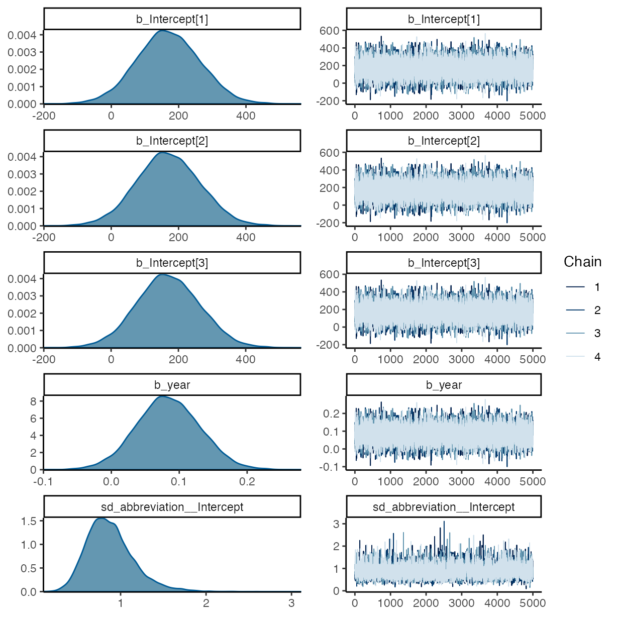


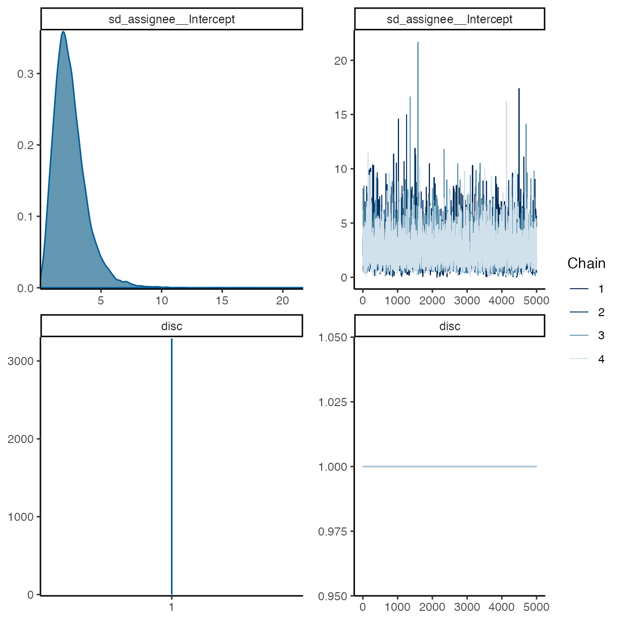
pp_check(m_g2, ndraws = 50, type = "bars")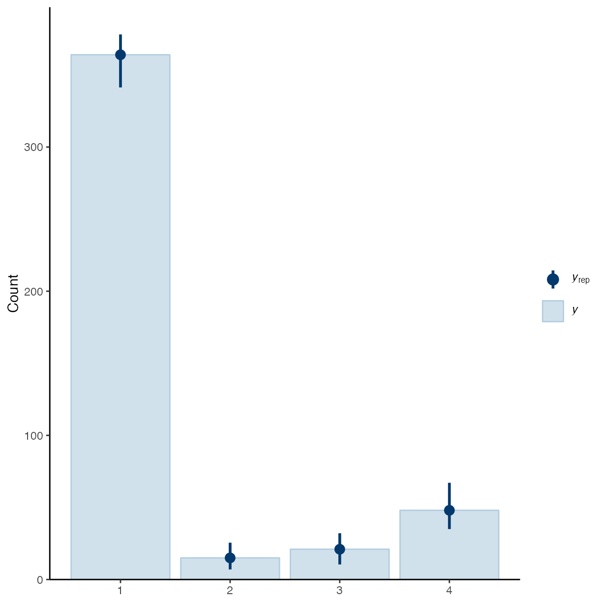


plot(equivalence_test(m_g2))
#> Picking joint bandwidth of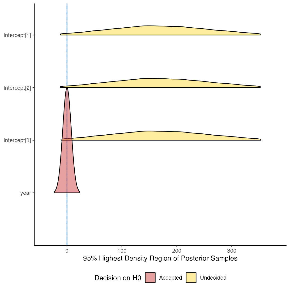 7.73
#> Warning: Removed 4000 rows containing non-finite values
#> (`stat_density_ridges()`).


pander(m_g2_report <- report(m_g2))
#> Warning: Predictions are treated as continuous variables in 'bayes_R2' which is
#> likely invalid for ordinal families.
#> Warning: Predictions are treated as continuous variables in 'bayes_R2' which is
#> likely invalid for ordinal families.
#> Start sampling
#> Warning: Predictions are treated as continuous variables in 'bayes_R2' which is
#> likely invalid for ordinal families.

#> Warning: Predictions are treated as continuous variables in 'bayes_R2' which is
#> likely invalid for ordinal families.

_We fitted a Bayesian logistic mixed model (estimated using MCMC sampling with 4 chains of 10000 iterations and a warmup of 5000) to predict data_avail with year (formula: data_avail ~ year). The model included abbreviation as random effects (formula: list(~1 | abbreviation, ~1 | assignee)). Priors over parameters were set as normal (mean = 0.00, SD = 1.00) distributions. The model’s explanatory power is weak (R2 = 0.11, 95% CI [0.05, 0.18]) and the part related to the fixed effects alone (marginal R2) is of 0.02 (95% CI [3.48e-10, 0.08]). Within this model:

The effect of b Intercept[1] (Median = 167.70, 95% CI [-15.45, 354.89]) has a 96.36% probability of being positive (> 0), 96.36% of being significant (> 0.05), and 96.34% of being large (> 0.30). The estimation successfully converged (Rhat = 1.000) and the indices are reliable (ESS = 25325)
The effect of b Intercept[2] (Median = 167.97, 95% CI [-15.23, 355.26]) has a 96.39% probability of being positive (> 0), 96.38% of being significant (> 0.05), and 96.36% of being large (> 0.30). The estimation successfully converged (Rhat = 1.000) and the indices are reliable (ESS = 25322)
The effect of b Intercept[3] (Median = 168.40, 95% CI [-14.72, 355.72]) has a 96.42% probability of being positive (> 0), 96.41% of being significant (> 0.05), and 96.40% of being large (> 0.30). The estimation successfully converged (Rhat = 1.000) and the indices are reliable (ESS = 25323)
The effect of b year (Median = 0.08, 95% CI [-7.81e-03, 0.18]) has a 96.36% probability of being positive (> 0), 76.55% of being significant (> 0.05), and 0.00% of being large (> 0.30). The estimation successfully converged (Rhat = 1.000) and the indices are reliable (ESS = 25157)

Following the Sequential Effect eXistence and sIgnificance Testing (SEXIT) framework, we report the median of the posterior distribution and its 95% CI (Highest Density Interval), along the probability of direction (pd), the probability of significance and the probability of being large. The thresholds beyond which the effect is considered as significant (i.e., non-negligible) and large are |0.05| and |0.30|. Convergence and stability of the Bayesian sampling has been assessed using R-hat, which should be below 1.01 (Vehtari et al., 2019), and Effective Sample Size (ESS), which should be greater than 1000 (Burkner, 2017)._, _We fitted a Bayesian logistic mixed model (estimated using MCMC sampling with 4 chains of 10000 iterations and a warmup of 5000) to predict data_avail with year (formula: data_avail ~ year). The model included abbreviation as random effects (formula: list(~1 | abbreviation, ~1 | assignee)). Priors over parameters were set as normal (mean = 0.00, SD = 1.00) distributions. The model’s explanatory power is weak (R2 = 0.11, 95% CI [0.05, 0.18]) and the part related to the fixed effects alone (marginal R2) is of 0.02 (95% CI [3.48e-10, 0.08]). Within this model:

The effect of b Intercept[1] (Median = 167.70, 95% CI [-15.45, 354.89]) has a 96.36% probability of being positive (> 0), 96.36% of being significant (> 0.05), and 96.34% of being large (> 0.30). The estimation successfully converged (Rhat = 1.000) and the indices are reliable (ESS = 25325)
The effect of b Intercept[2] (Median = 167.97, 95% CI [-15.23, 355.26]) has a 96.39% probability of being positive (> 0), 96.38% of being significant (> 0.05), and 96.36% of being large (> 0.30). The estimation successfully converged (Rhat = 1.000) and the indices are reliable (ESS = 25322)
The effect of b Intercept[3] (Median = 168.40, 95% CI [-14.72, 355.72]) has a 96.42% probability of being positive (> 0), 96.41% of being significant (> 0.05), and 96.40% of being large (> 0.30). The estimation successfully converged (Rhat = 1.000) and the indices are reliable (ESS = 25323)
The effect of b year (Median = 0.08, 95% CI [-7.81e-03, 0.18]) has a 96.36% probability of being positive (> 0), 76.55% of being significant (> 0.05), and 0.00% of being large (> 0.30). The estimation successfully converged (Rhat = 1.000) and the indices are reliable (ESS = 25157)

Following the Sequential Effect eXistence and sIgnificance Testing (SEXIT) framework, we report the median of the posterior distribution and its 95% CI (Highest Density Interval), along the probability of direction (pd), the probability of significance and the probability of being large. The thresholds beyond which the effect is considered as significant (i.e., non-negligible) and large are |0.05| and |0.30|. Convergence and stability of the Bayesian sampling has been assessed using R-hat, which should be below 1.01 (Vehtari et al., 2019), and Effective Sample Size (ESS), which should be greater than 1000 (Burkner, 2017)._, _We fitted a Bayesian logistic mixed model (estimated using MCMC sampling with 4 chains of 10000 iterations and a warmup of 5000) to predict data_avail with year (formula: data_avail ~ year). The model included abbreviation as random effects (formula: list(~1 | abbreviation, ~1 | assignee)). Priors over parameters were set as normal (mean = 0.00, SD = 1.00) distributions. The model’s explanatory power is weak (R2 = 0.11, 95% CI [0.05, 0.18]) and the part related to the fixed effects alone (marginal R2) is of 0.02 (95% CI [3.48e-10, 0.08]). Within this model:

The effect of b Intercept[1] (Median = 167.70, 95% CI [-15.45, 354.89]) has a 96.36% probability of being positive (> 0), 96.36% of being significant (> 0.05), and 96.34% of being large (> 0.30). The estimation successfully converged (Rhat = 1.000) and the indices are reliable (ESS = 25325)
The effect of b Intercept[2] (Median = 167.97, 95% CI [-15.23, 355.26]) has a 96.39% probability of being positive (> 0), 96.38% of being significant (> 0.05), and 96.36% of being large (> 0.30). The estimation successfully converged (Rhat = 1.000) and the indices are reliable (ESS = 25322)
The effect of b Intercept[3] (Median = 168.40, 95% CI [-14.72, 355.72]) has a 96.42% probability of being positive (> 0), 96.41% of being significant (> 0.05), and 96.40% of being large (> 0.30). The estimation successfully converged (Rhat = 1.000) and the indices are reliable (ESS = 25323)
The effect of b year (Median = 0.08, 95% CI [-7.81e-03, 0.18]) has a 96.36% probability of being positive (> 0), 76.55% of being significant (> 0.05), and 0.00% of being large (> 0.30). The estimation successfully converged (Rhat = 1.000) and the indices are reliable (ESS = 25157)

Following the Sequential Effect eXistence and sIgnificance Testing (SEXIT) framework, we report the median of the posterior distribution and its 95% CI (Highest Density Interval), along the probability of direction (pd), the probability of significance and the probability of being large. The thresholds beyond which the effect is considered as significant (i.e., non-negligible) and large are |0.05| and |0.30|. Convergence and stability of the Bayesian sampling has been assessed using R-hat, which should be below 1.01 (Vehtari et al., 2019), and Effective Sample Size (ESS), which should be greater than 1000 (Burkner, 2017)._, _We fitted a Bayesian logistic mixed model (estimated using MCMC sampling with 4 chains of 10000 iterations and a warmup of 5000) to predict data_avail with year (formula: data_avail ~ year). The model included abbreviation as random effects (formula: list(~1 | abbreviation, ~1 | assignee)). Priors over parameters were set as normal (mean = 0.00, SD = 1.00) distributions. The model’s explanatory power is weak (R2 = 0.11, 95% CI [0.05, 0.18]) and the part related to the fixed effects alone (marginal R2) is of 0.02 (95% CI [3.48e-10, 0.08]). Within this model:

The effect of b Intercept[1] (Median = 167.70, 95% CI [-15.45, 354.89]) has a 96.36% probability of being positive (> 0), 96.36% of being significant (> 0.05), and 96.34% of being large (> 0.30). The estimation successfully converged (Rhat = 1.000) and the indices are reliable (ESS = 25325)
The effect of b Intercept[2] (Median = 167.97, 95% CI [-15.23, 355.26]) has a 96.39% probability of being positive (> 0), 96.38% of being significant (> 0.05), and 96.36% of being large (> 0.30). The estimation successfully converged (Rhat = 1.000) and the indices are reliable (ESS = 25322)
The effect of b Intercept[3] (Median = 168.40, 95% CI [-14.72, 355.72]) has a 96.42% probability of being positive (> 0), 96.41% of being significant (> 0.05), and 96.40% of being large (> 0.30). The estimation successfully converged (Rhat = 1.000) and the indices are reliable (ESS = 25323)
The effect of b year (Median = 0.08, 95% CI [-7.81e-03, 0.18]) has a 96.36% probability of being positive (> 0), 76.55% of being significant (> 0.05), and 0.00% of being large (> 0.30). The estimation successfully converged (Rhat = 1.000) and the indices are reliable (ESS = 25157)

Following the Sequential Effect eXistence and sIgnificance Testing (SEXIT) framework, we report the median of the posterior distribution and its 95% CI (Highest Density Interval), along the probability of direction (pd), the probability of significance and the probability of being large. The thresholds beyond which the effect is considered as significant (i.e., non-negligible) and large are |0.05| and |0.30|. Convergence and stability of the Bayesian sampling has been assessed using R-hat, which should be below 1.01 (Vehtari et al., 2019), and Effective Sample Size (ESS), which should be greater than 1000 (Burkner, 2017)._, _We fitted a Bayesian logistic mixed model (estimated using MCMC sampling with 4 chains of 10000 iterations and a warmup of 5000) to predict data_avail with year (formula: data_avail ~ year). The model included abbreviation as random effects (formula: list(~1 | abbreviation, ~1 | assignee)). Priors over parameters were set as normal (mean = 0.00, SD = 1.00) distributions. The model’s explanatory power is weak (R2 = 0.11, 95% CI [0.05, 0.18]) and the part related to the fixed effects alone (marginal R2) is of 0.02 (95% CI [3.48e-10, 0.08]). Within this model:

The effect of b Intercept[1] (Median = 167.70, 95% CI [-15.45, 354.89]) has a 96.36% probability of being positive (> 0), 96.36% of being significant (> 0.05), and 96.34% of being large (> 0.30). The estimation successfully converged (Rhat = 1.000) and the indices are reliable (ESS = 25325)
The effect of b Intercept[2] (Median = 167.97, 95% CI [-15.23, 355.26]) has a 96.39% probability of being positive (> 0), 96.38% of being significant (> 0.05), and 96.36% of being large (> 0.30). The estimation successfully converged (Rhat = 1.000) and the indices are reliable (ESS = 25322)
The effect of b Intercept[3] (Median = 168.40, 95% CI [-14.72, 355.72]) has a 96.42% probability of being positive (> 0), 96.41% of being significant (> 0.05), and 96.40% of being large (> 0.30). The estimation successfully converged (Rhat = 1.000) and the indices are reliable (ESS = 25323)
The effect of b year (Median = 0.08, 95% CI [-7.81e-03, 0.18]) has a 96.36% probability of being positive (> 0), 76.55% of being significant (> 0.05), and 0.00% of being large (> 0.30). The estimation successfully converged (Rhat = 1.000) and the indices are reliable (ESS = 25157)

Following the Sequential Effect eXistence and sIgnificance Testing (SEXIT) framework, we report the median of the posterior distribution and its 95% CI (Highest Density Interval), along the probability of direction (pd), the probability of significance and the probability of being large. The thresholds beyond which the effect is considered as significant (i.e., non-negligible) and large are |0.05| and |0.30|. Convergence and stability of the Bayesian sampling has been assessed using R-hat, which should be below 1.01 (Vehtari et al., 2019), and Effective Sample Size (ESS), which should be greater than 1000 (Burkner, 2017)._, _We fitted a Bayesian logistic mixed model (estimated using MCMC sampling with 4 chains of 10000 iterations and a warmup of 5000) to predict data_avail with year (formula: data_avail ~ year). The model included abbreviation as random effects (formula: list(~1 | abbreviation, ~1 | assignee)). Priors over parameters were set as normal (mean = 0.00, SD = 1.00) distributions. The model’s explanatory power is weak (R2 = 0.11, 95% CI [0.05, 0.18]) and the part related to the fixed effects alone (marginal R2) is of 0.02 (95% CI [3.48e-10, 0.08]). Within this model:

The effect of b Intercept[1] (Median = 167.70, 95% CI [-15.45, 354.89]) has a 96.36% probability of being positive (> 0), 96.36% of being significant (> 0.05), and 96.34% of being large (> 0.30). The estimation successfully converged (Rhat = 1.000) and the indices are reliable (ESS = 25325)
The effect of b Intercept[2] (Median = 167.97, 95% CI [-15.23, 355.26]) has a 96.39% probability of being positive (> 0), 96.38% of being significant (> 0.05), and 96.36% of being large (> 0.30). The estimation successfully converged (Rhat = 1.000) and the indices are reliable (ESS = 25322)
The effect of b Intercept[3] (Median = 168.40, 95% CI [-14.72, 355.72]) has a 96.42% probability of being positive (> 0), 96.41% of being significant (> 0.05), and 96.40% of being large (> 0.30). The estimation successfully converged (Rhat = 1.000) and the indices are reliable (ESS = 25323)
The effect of b year (Median = 0.08, 95% CI [-7.81e-03, 0.18]) has a 96.36% probability of being positive (> 0), 76.55% of being significant (> 0.05), and 0.00% of being large (> 0.30). The estimation successfully converged (Rhat = 1.000) and the indices are reliable (ESS = 25157)

Following the Sequential Effect eXistence and sIgnificance Testing (SEXIT) framework, we report the median of the posterior distribution and its 95% CI (Highest Density Interval), along the probability of direction (pd), the probability of significance and the probability of being large. The thresholds beyond which the effect is considered as significant (i.e., non-negligible) and large are |0.05| and |0.30|. Convergence and stability of the Bayesian sampling has been assessed using R-hat, which should be below 1.01 (Vehtari et al., 2019), and Effective Sample Size (ESS), which should be greater than 1000 (Burkner, 2017)._, _We fitted a Bayesian logistic mixed model (estimated using MCMC sampling with 4 chains of 10000 iterations and a warmup of 5000) to predict data_avail with year (formula: data_avail ~ year). The model included abbreviation as random effects (formula: list(~1 | abbreviation, ~1 | assignee)). Priors over parameters were set as normal (mean = 0.00, SD = 1.00) distributions. The model’s explanatory power is weak (R2 = 0.11, 95% CI [0.05, 0.18]) and the part related to the fixed effects alone (marginal R2) is of 0.02 (95% CI [3.48e-10, 0.08]). Within this model:

The effect of b Intercept[1] (Median = 167.70, 95% CI [-15.45, 354.89]) has a 96.36% probability of being positive (> 0), 96.36% of being significant (> 0.05), and 96.34% of being large (> 0.30). The estimation successfully converged (Rhat = 1.000) and the indices are reliable (ESS = 25325)
The effect of b Intercept[2] (Median = 167.97, 95% CI [-15.23, 355.26]) has a 96.39% probability of being positive (> 0), 96.38% of being significant (> 0.05), and 96.36% of being large (> 0.30). The estimation successfully converged (Rhat = 1.000) and the indices are reliable (ESS = 25322)
The effect of b Intercept[3] (Median = 168.40, 95% CI [-14.72, 355.72]) has a 96.42% probability of being positive (> 0), 96.41% of being significant (> 0.05), and 96.40% of being large (> 0.30). The estimation successfully converged (Rhat = 1.000) and the indices are reliable (ESS = 25323)
The effect of b year (Median = 0.08, 95% CI [-7.81e-03, 0.18]) has a 96.36% probability of being positive (> 0), 76.55% of being significant (> 0.05), and 0.00% of being large (> 0.30). The estimation successfully converged (Rhat = 1.000) and the indices are reliable (ESS = 25157)

Following the Sequential Effect eXistence and sIgnificance Testing (SEXIT) framework, we report the median of the posterior distribution and its 95% CI (Highest Density Interval), along the probability of direction (pd), the probability of significance and the probability of being large. The thresholds beyond which the effect is considered as significant (i.e., non-negligible) and large are |0.05| and |0.30|. Convergence and stability of the Bayesian sampling has been assessed using R-hat, which should be below 1.01 (Vehtari et al., 2019), and Effective Sample Size (ESS), which should be greater than 1000 (Burkner, 2017)._, _We fitted a Bayesian logistic mixed model (estimated using MCMC sampling with 4 chains of 10000 iterations and a warmup of 5000) to predict data_avail with year (formula: data_avail ~ year). The model included abbreviation as random effects (formula: list(~1 | abbreviation, ~1 | assignee)). Priors over parameters were set as normal (mean = 0.00, SD = 1.00) distributions. The model’s explanatory power is weak (R2 = 0.11, 95% CI [0.05, 0.18]) and the part related to the fixed effects alone (marginal R2) is of 0.02 (95% CI [3.48e-10, 0.08]). Within this model:

The effect of b Intercept[1] (Median = 167.70, 95% CI [-15.45, 354.89]) has a 96.36% probability of being positive (> 0), 96.36% of being significant (> 0.05), and 96.34% of being large (> 0.30). The estimation successfully converged (Rhat = 1.000) and the indices are reliable (ESS = 25325)
The effect of b Intercept[2] (Median = 167.97, 95% CI [-15.23, 355.26]) has a 96.39% probability of being positive (> 0), 96.38% of being significant (> 0.05), and 96.36% of being large (> 0.30). The estimation successfully converged (Rhat = 1.000) and the indices are reliable (ESS = 25322)
The effect of b Intercept[3] (Median = 168.40, 95% CI [-14.72, 355.72]) has a 96.42% probability of being positive (> 0), 96.41% of being significant (> 0.05), and 96.40% of being large (> 0.30). The estimation successfully converged (Rhat = 1.000) and the indices are reliable (ESS = 25323)
The effect of b year (Median = 0.08, 95% CI [-7.81e-03, 0.18]) has a 96.36% probability of being positive (> 0), 76.55% of being significant (> 0.05), and 0.00% of being large (> 0.30). The estimation successfully converged (Rhat = 1.000) and the indices are reliable (ESS = 25157)

Following the Sequential Effect eXistence and sIgnificance Testing (SEXIT) framework, we report the median of the posterior distribution and its 95% CI (Highest Density Interval), along the probability of direction (pd), the probability of significance and the probability of being large. The thresholds beyond which the effect is considered as significant (i.e., non-negligible) and large are |0.05| and |0.30|. Convergence and stability of the Bayesian sampling has been assessed using R-hat, which should be below 1.01 (Vehtari et al., 2019), and Effective Sample Size (ESS), which should be greater than 1000 (Burkner, 2017)._, _We fitted a Bayesian logistic mixed model (estimated using MCMC sampling with 4 chains of 10000 iterations and a warmup of 5000) to predict data_avail with year (formula: data_avail ~ year). The model included abbreviation as random effects (formula: list(~1 | abbreviation, ~1 | assignee)). Priors over parameters were set as normal (mean = 0.00, SD = 1.00) distributions. The model’s explanatory power is weak (R2 = 0.11, 95% CI [0.05, 0.18]) and the part related to the fixed effects alone (marginal R2) is of 0.02 (95% CI [3.48e-10, 0.08]). Within this model:

The effect of b Intercept[1] (Median = 167.70, 95% CI [-15.45, 354.89]) has a 96.36% probability of being positive (> 0), 96.36% of being significant (> 0.05), and 96.34% of being large (> 0.30). The estimation successfully converged (Rhat = 1.000) and the indices are reliable (ESS = 25325)
The effect of b Intercept[2] (Median = 167.97, 95% CI [-15.23, 355.26]) has a 96.39% probability of being positive (> 0), 96.38% of being significant (> 0.05), and 96.36% of being large (> 0.30). The estimation successfully converged (Rhat = 1.000) and the indices are reliable (ESS = 25322)
The effect of b Intercept[3] (Median = 168.40, 95% CI [-14.72, 355.72]) has a 96.42% probability of being positive (> 0), 96.41% of being significant (> 0.05), and 96.40% of being large (> 0.30). The estimation successfully converged (Rhat = 1.000) and the indices are reliable (ESS = 25323)
The effect of b year (Median = 0.08, 95% CI [-7.81e-03, 0.18]) has a 96.36% probability of being positive (> 0), 76.55% of being significant (> 0.05), and 0.00% of being large (> 0.30). The estimation successfully converged (Rhat = 1.000) and the indices are reliable (ESS = 25157)

Following the Sequential Effect eXistence and sIgnificance Testing (SEXIT) framework, we report the median of the posterior distribution and its 95% CI (Highest Density Interval), along the probability of direction (pd), the probability of significance and the probability of being large. The thresholds beyond which the effect is considered as significant (i.e., non-negligible) and large are |0.05| and |0.30|. Convergence and stability of the Bayesian sampling has been assessed using R-hat, which should be below 1.01 (Vehtari et al., 2019), and Effective Sample Size (ESS), which should be greater than 1000 (Burkner, 2017)._, _We fitted a Bayesian logistic mixed model (estimated using MCMC sampling with 4 chains of 10000 iterations and a warmup of 5000) to predict data_avail with year (formula: data_avail ~ year). The model included abbreviation as random effects (formula: list(~1 | abbreviation, ~1 | assignee)). Priors over parameters were set as normal (mean = 0.00, SD = 1.00) distributions. The model’s explanatory power is weak (R2 = 0.11, 95% CI [0.05, 0.18]) and the part related to the fixed effects alone (marginal R2) is of 0.02 (95% CI [3.48e-10, 0.08]). Within this model:

The effect of b Intercept[1] (Median = 167.70, 95% CI [-15.45, 354.89]) has a 96.36% probability of being positive (> 0), 96.36% of being significant (> 0.05), and 96.34% of being large (> 0.30). The estimation successfully converged (Rhat = 1.000) and the indices are reliable (ESS = 25325)
The effect of b Intercept[2] (Median = 167.97, 95% CI [-15.23, 355.26]) has a 96.39% probability of being positive (> 0), 96.38% of being significant (> 0.05), and 96.36% of being large (> 0.30). The estimation successfully converged (Rhat = 1.000) and the indices are reliable (ESS = 25322)
The effect of b Intercept[3] (Median = 168.40, 95% CI [-14.72, 355.72]) has a 96.42% probability of being positive (> 0), 96.41% of being significant (> 0.05), and 96.40% of being large (> 0.30). The estimation successfully converged (Rhat = 1.000) and the indices are reliable (ESS = 25323)
The effect of b year (Median = 0.08, 95% CI [-7.81e-03, 0.18]) has a 96.36% probability of being positive (> 0), 76.55% of being significant (> 0.05), and 0.00% of being large (> 0.30). The estimation successfully converged (Rhat = 1.000) and the indices are reliable (ESS = 25157)

Following the Sequential Effect eXistence and sIgnificance Testing (SEXIT) framework, we report the median of the posterior distribution and its 95% CI (Highest Density Interval), along the probability of direction (pd), the probability of significance and the probability of being large. The thresholds beyond which the effect is considered as significant (i.e., non-negligible) and large are |0.05| and |0.30|. Convergence and stability of the Bayesian sampling has been assessed using R-hat, which should be below 1.01 (Vehtari et al., 2019), and Effective Sample Size (ESS), which should be greater than 1000 (Burkner, 2017)._, _We fitted a Bayesian logistic mixed model (estimated using MCMC sampling with 4 chains of 10000 iterations and a warmup of 5000) to predict data_avail with year (formula: data_avail ~ year). The model included abbreviation as random effects (formula: list(~1 | abbreviation, ~1 | assignee)). Priors over parameters were set as normal (mean = 0.00, SD = 1.00) distributions. The model’s explanatory power is weak (R2 = 0.11, 95% CI [0.05, 0.18]) and the part related to the fixed effects alone (marginal R2) is of 0.02 (95% CI [3.48e-10, 0.08]). Within this model:

The effect of b Intercept[1] (Median = 167.70, 95% CI [-15.45, 354.89]) has a 96.36% probability of being positive (> 0), 96.36% of being significant (> 0.05), and 96.34% of being large (> 0.30). The estimation successfully converged (Rhat = 1.000) and the indices are reliable (ESS = 25325)
The effect of b Intercept[2] (Median = 167.97, 95% CI [-15.23, 355.26]) has a 96.39% probability of being positive (> 0), 96.38% of being significant (> 0.05), and 96.36% of being large (> 0.30). The estimation successfully converged (Rhat = 1.000) and the indices are reliable (ESS = 25322)
The effect of b Intercept[3] (Median = 168.40, 95% CI [-14.72, 355.72]) has a 96.42% probability of being positive (> 0), 96.41% of being significant (> 0.05), and 96.40% of being large (> 0.30). The estimation successfully converged (Rhat = 1.000) and the indices are reliable (ESS = 25323)
The effect of b year (Median = 0.08, 95% CI [-7.81e-03, 0.18]) has a 96.36% probability of being positive (> 0), 76.55% of being significant (> 0.05), and 0.00% of being large (> 0.30). The estimation successfully converged (Rhat = 1.000) and the indices are reliable (ESS = 25157)

Following the Sequential Effect eXistence and sIgnificance Testing (SEXIT) framework, we report the median of the posterior distribution and its 95% CI (Highest Density Interval), along the probability of direction (pd), the probability of significance and the probability of being large. The thresholds beyond which the effect is considered as significant (i.e., non-negligible) and large are |0.05| and |0.30|. Convergence and stability of the Bayesian sampling has been assessed using R-hat, which should be below 1.01 (Vehtari et al., 2019), and Effective Sample Size (ESS), which should be greater than 1000 (Burkner, 2017)._, _We fitted a Bayesian logistic mixed model (estimated using MCMC sampling with 4 chains of 10000 iterations and a warmup of 5000) to predict data_avail with year (formula: data_avail ~ year). The model included abbreviation as random effects (formula: list(~1 | abbreviation, ~1 | assignee)). Priors over parameters were set as normal (mean = 0.00, SD = 1.00) distributions. The model’s explanatory power is weak (R2 = 0.11, 95% CI [0.05, 0.18]) and the part related to the fixed effects alone (marginal R2) is of 0.02 (95% CI [3.48e-10, 0.08]). Within this model:

The effect of b Intercept[1] (Median = 167.70, 95% CI [-15.45, 354.89]) has a 96.36% probability of being positive (> 0), 96.36% of being significant (> 0.05), and 96.34% of being large (> 0.30). The estimation successfully converged (Rhat = 1.000) and the indices are reliable (ESS = 25325)
The effect of b Intercept[2] (Median = 167.97, 95% CI [-15.23, 355.26]) has a 96.39% probability of being positive (> 0), 96.38% of being significant (> 0.05), and 96.36% of being large (> 0.30). The estimation successfully converged (Rhat = 1.000) and the indices are reliable (ESS = 25322)
The effect of b Intercept[3] (Median = 168.40, 95% CI [-14.72, 355.72]) has a 96.42% probability of being positive (> 0), 96.41% of being significant (> 0.05), and 96.40% of being large (> 0.30). The estimation successfully converged (Rhat = 1.000) and the indices are reliable (ESS = 25323)
The effect of b year (Median = 0.08, 95% CI [-7.81e-03, 0.18]) has a 96.36% probability of being positive (> 0), 76.55% of being significant (> 0.05), and 0.00% of being large (> 0.30). The estimation successfully converged (Rhat = 1.000) and the indices are reliable (ESS = 25157)

Following the Sequential Effect eXistence and sIgnificance Testing (SEXIT) framework, we report the median of the posterior distribution and its 95% CI (Highest Density Interval), along the probability of direction (pd), the probability of significance and the probability of being large. The thresholds beyond which the effect is considered as significant (i.e., non-negligible) and large are |0.05| and |0.30|. Convergence and stability of the Bayesian sampling has been assessed using R-hat, which should be below 1.01 (Vehtari et al., 2019), and Effective Sample Size (ESS), which should be greater than 1000 (Burkner, 2017)._, _We fitted a Bayesian logistic mixed model (estimated using MCMC sampling with 4 chains of 10000 iterations and a warmup of 5000) to predict data_avail with year (formula: data_avail ~ year). The model included abbreviation as random effects (formula: list(~1 | abbreviation, ~1 | assignee)). Priors over parameters were set as normal (mean = 0.00, SD = 1.00) distributions. The model’s explanatory power is weak (R2 = 0.11, 95% CI [0.05, 0.18]) and the part related to the fixed effects alone (marginal R2) is of 0.02 (95% CI [3.48e-10, 0.08]). Within this model:

The effect of b Intercept[1] (Median = 167.70, 95% CI [-15.45, 354.89]) has a 96.36% probability of being positive (> 0), 96.36% of being significant (> 0.05), and 96.34% of being large (> 0.30). The estimation successfully converged (Rhat = 1.000) and the indices are reliable (ESS = 25325)
The effect of b Intercept[2] (Median = 167.97, 95% CI [-15.23, 355.26]) has a 96.39% probability of being positive (> 0), 96.38% of being significant (> 0.05), and 96.36% of being large (> 0.30). The estimation successfully converged (Rhat = 1.000) and the indices are reliable (ESS = 25322)
The effect of b Intercept[3] (Median = 168.40, 95% CI [-14.72, 355.72]) has a 96.42% probability of being positive (> 0), 96.41% of being significant (> 0.05), and 96.40% of being large (> 0.30). The estimation successfully converged (Rhat = 1.000) and the indices are reliable (ESS = 25323)
The effect of b year (Median = 0.08, 95% CI [-7.81e-03, 0.18]) has a 96.36% probability of being positive (> 0), 76.55% of being significant (> 0.05), and 0.00% of being large (> 0.30). The estimation successfully converged (Rhat = 1.000) and the indices are reliable (ESS = 25157)

Following the Sequential Effect eXistence and sIgnificance Testing (SEXIT) framework, we report the median of the posterior distribution and its 95% CI (Highest Density Interval), along the probability of direction (pd), the probability of significance and the probability of being large. The thresholds beyond which the effect is considered as significant (i.e., non-negligible) and large are |0.05| and |0.30|. Convergence and stability of the Bayesian sampling has been assessed using R-hat, which should be below 1.01 (Vehtari et al., 2019), and Effective Sample Size (ESS), which should be greater than 1000 (Burkner, 2017)._, _We fitted a Bayesian logistic mixed model (estimated using MCMC sampling with 4 chains of 10000 iterations and a warmup of 5000) to predict data_avail with year (formula: data_avail ~ year). The model included abbreviation as random effects (formula: list(~1 | abbreviation, ~1 | assignee)). Priors over parameters were set as normal (mean = 0.00, SD = 1.00) distributions. The model’s explanatory power is weak (R2 = 0.11, 95% CI [0.05, 0.18]) and the part related to the fixed effects alone (marginal R2) is of 0.02 (95% CI [3.48e-10, 0.08]). Within this model:

The effect of b Intercept[1] (Median = 167.70, 95% CI [-15.45, 354.89]) has a 96.36% probability of being positive (> 0), 96.36% of being significant (> 0.05), and 96.34% of being large (> 0.30). The estimation successfully converged (Rhat = 1.000) and the indices are reliable (ESS = 25325)
The effect of b Intercept[2] (Median = 167.97, 95% CI [-15.23, 355.26]) has a 96.39% probability of being positive (> 0), 96.38% of being significant (> 0.05), and 96.36% of being large (> 0.30). The estimation successfully converged (Rhat = 1.000) and the indices are reliable (ESS = 25322)
The effect of b Intercept[3] (Median = 168.40, 95% CI [-14.72, 355.72]) has a 96.42% probability of being positive (> 0), 96.41% of being significant (> 0.05), and 96.40% of being large (> 0.30). The estimation successfully converged (Rhat = 1.000) and the indices are reliable (ESS = 25323)
The effect of b year (Median = 0.08, 95% CI [-7.81e-03, 0.18]) has a 96.36% probability of being positive (> 0), 76.55% of being significant (> 0.05), and 0.00% of being large (> 0.30). The estimation successfully converged (Rhat = 1.000) and the indices are reliable (ESS = 25157)

Following the Sequential Effect eXistence and sIgnificance Testing (SEXIT) framework, we report the median of the posterior distribution and its 95% CI (Highest Density Interval), along the probability of direction (pd), the probability of significance and the probability of being large. The thresholds beyond which the effect is considered as significant (i.e., non-negligible) and large are |0.05| and |0.30|. Convergence and stability of the Bayesian sampling has been assessed using R-hat, which should be below 1.01 (Vehtari et al., 2019), and Effective Sample Size (ESS), which should be greater than 1000 (Burkner, 2017)._, _We fitted a Bayesian logistic mixed model (estimated using MCMC sampling with 4 chains of 10000 iterations and a warmup of 5000) to predict data_avail with year (formula: data_avail ~ year). The model included abbreviation as random effects (formula: list(~1 | abbreviation, ~1 | assignee)). Priors over parameters were set as normal (mean = 0.00, SD = 1.00) distributions. The model’s explanatory power is weak (R2 = 0.11, 95% CI [0.05, 0.18]) and the part related to the fixed effects alone (marginal R2) is of 0.02 (95% CI [3.48e-10, 0.08]). Within this model:

The effect of b Intercept[1] (Median = 167.70, 95% CI [-15.45, 354.89]) has a 96.36% probability of being positive (> 0), 96.36% of being significant (> 0.05), and 96.34% of being large (> 0.30). The estimation successfully converged (Rhat = 1.000) and the indices are reliable (ESS = 25325)
The effect of b Intercept[2] (Median = 167.97, 95% CI [-15.23, 355.26]) has a 96.39% probability of being positive (> 0), 96.38% of being significant (> 0.05), and 96.36% of being large (> 0.30). The estimation successfully converged (Rhat = 1.000) and the indices are reliable (ESS = 25322)
The effect of b Intercept[3] (Median = 168.40, 95% CI [-14.72, 355.72]) has a 96.42% probability of being positive (> 0), 96.41% of being significant (> 0.05), and 96.40% of being large (> 0.30). The estimation successfully converged (Rhat = 1.000) and the indices are reliable (ESS = 25323)
The effect of b year (Median = 0.08, 95% CI [-7.81e-03, 0.18]) has a 96.36% probability of being positive (> 0), 76.55% of being significant (> 0.05), and 0.00% of being large (> 0.30). The estimation successfully converged (Rhat = 1.000) and the indices are reliable (ESS = 25157)

Following the Sequential Effect eXistence and sIgnificance Testing (SEXIT) framework, we report the median of the posterior distribution and its 95% CI (Highest Density Interval), along the probability of direction (pd), the probability of significance and the probability of being large. The thresholds beyond which the effect is considered as significant (i.e., non-negligible) and large are |0.05| and |0.30|. Convergence and stability of the Bayesian sampling has been assessed using R-hat, which should be below 1.01 (Vehtari et al., 2019), and Effective Sample Size (ESS), which should be greater than 1000 (Burkner, 2017)._, _We fitted a Bayesian logistic mixed model (estimated using MCMC sampling with 4 chains of 10000 iterations and a warmup of 5000) to predict data_avail with year (formula: data_avail ~ year). The model included abbreviation as random effects (formula: list(~1 | abbreviation, ~1 | assignee)). Priors over parameters were set as normal (mean = 0.00, SD = 1.00) distributions. The model’s explanatory power is weak (R2 = 0.11, 95% CI [0.05, 0.18]) and the part related to the fixed effects alone (marginal R2) is of 0.02 (95% CI [3.48e-10, 0.08]). Within this model:

The effect of b Intercept[1] (Median = 167.70, 95% CI [-15.45, 354.89]) has a 96.36% probability of being positive (> 0), 96.36% of being significant (> 0.05), and 96.34% of being large (> 0.30). The estimation successfully converged (Rhat = 1.000) and the indices are reliable (ESS = 25325)
The effect of b Intercept[2] (Median = 167.97, 95% CI [-15.23, 355.26]) has a 96.39% probability of being positive (> 0), 96.38% of being significant (> 0.05), and 96.36% of being large (> 0.30). The estimation successfully converged (Rhat = 1.000) and the indices are reliable (ESS = 25322)
The effect of b Intercept[3] (Median = 168.40, 95% CI [-14.72, 355.72]) has a 96.42% probability of being positive (> 0), 96.41% of being significant (> 0.05), and 96.40% of being large (> 0.30). The estimation successfully converged (Rhat = 1.000) and the indices are reliable (ESS = 25323)
The effect of b year (Median = 0.08, 95% CI [-7.81e-03, 0.18]) has a 96.36% probability of being positive (> 0), 76.55% of being significant (> 0.05), and 0.00% of being large (> 0.30). The estimation successfully converged (Rhat = 1.000) and the indices are reliable (ESS = 25157)

Following the Sequential Effect eXistence and sIgnificance Testing (SEXIT) framework, we report the median of the posterior distribution and its 95% CI (Highest Density Interval), along the probability of direction (pd), the probability of significance and the probability of being large. The thresholds beyond which the effect is considered as significant (i.e., non-negligible) and large are |0.05| and |0.30|. Convergence and stability of the Bayesian sampling has been assessed using R-hat, which should be below 1.01 (Vehtari et al., 2019), and Effective Sample Size (ESS), which should be greater than 1000 (Burkner, 2017)._, _We fitted a Bayesian logistic mixed model (estimated using MCMC sampling with 4 chains of 10000 iterations and a warmup of 5000) to predict data_avail with year (formula: data_avail ~ year). The model included abbreviation as random effects (formula: list(~1 | abbreviation, ~1 | assignee)). Priors over parameters were set as student_t (location = 0.00, scale = 2.50) distributions. The model’s explanatory power is weak (R2 = 0.11, 95% CI [0.05, 0.18]) and the part related to the fixed effects alone (marginal R2) is of 0.02 (95% CI [3.48e-10, 0.08]). Within this model:

The effect of b Intercept[1] (Median = 167.70, 95% CI [-15.45, 354.89]) has a 96.36% probability of being positive (> 0), 96.36% of being significant (> 0.05), and 96.34% of being large (> 0.30). The estimation successfully converged (Rhat = 1.000) and the indices are reliable (ESS = 25325)
The effect of b Intercept[2] (Median = 167.97, 95% CI [-15.23, 355.26]) has a 96.39% probability of being positive (> 0), 96.38% of being significant (> 0.05), and 96.36% of being large (> 0.30). The estimation successfully converged (Rhat = 1.000) and the indices are reliable (ESS = 25322)
The effect of b Intercept[3] (Median = 168.40, 95% CI [-14.72, 355.72]) has a 96.42% probability of being positive (> 0), 96.41% of being significant (> 0.05), and 96.40% of being large (> 0.30). The estimation successfully converged (Rhat = 1.000) and the indices are reliable (ESS = 25323)
The effect of b year (Median = 0.08, 95% CI [-7.81e-03, 0.18]) has a 96.36% probability of being positive (> 0), 76.55% of being significant (> 0.05), and 0.00% of being large (> 0.30). The estimation successfully converged (Rhat = 1.000) and the indices are reliable (ESS = 25157)

Following the Sequential Effect eXistence and sIgnificance Testing (SEXIT) framework, we report the median of the posterior distribution and its 95% CI (Highest Density Interval), along the probability of direction (pd), the probability of significance and the probability of being large. The thresholds beyond which the effect is considered as significant (i.e., non-negligible) and large are |0.05| and |0.30|. Convergence and stability of the Bayesian sampling has been assessed using R-hat, which should be below 1.01 (Vehtari et al., 2019), and Effective Sample Size (ESS), which should be greater than 1000 (Burkner, 2017)._ and _We fitted a Bayesian logistic mixed model (estimated using MCMC sampling with 4 chains of 10000 iterations and a warmup of 5000) to predict data_avail with year (formula: data_avail ~ year). The model included abbreviation as random effects (formula: list(~1 | abbreviation, ~1 | assignee)). Priors over parameters were set as student_t (location = 0.00, scale = 2.50) distributions. The model’s explanatory power is weak (R2 = 0.11, 95% CI [0.05, 0.18]) and the part related to the fixed effects alone (marginal R2) is of 0.02 (95% CI [3.48e-10, 0.08]). Within this model:

The effect of b Intercept[1] (Median = 167.70, 95% CI [-15.45, 354.89]) has a 96.36% probability of being positive (> 0), 96.36% of being significant (> 0.05), and 96.34% of being large (> 0.30). The estimation successfully converged (Rhat = 1.000) and the indices are reliable (ESS = 25325)
The effect of b Intercept[2] (Median = 167.97, 95% CI [-15.23, 355.26]) has a 96.39% probability of being positive (> 0), 96.38% of being significant (> 0.05), and 96.36% of being large (> 0.30). The estimation successfully converged (Rhat = 1.000) and the indices are reliable (ESS = 25322)
The effect of b Intercept[3] (Median = 168.40, 95% CI [-14.72, 355.72]) has a 96.42% probability of being positive (> 0), 96.41% of being significant (> 0.05), and 96.40% of being large (> 0.30). The estimation successfully converged (Rhat = 1.000) and the indices are reliable (ESS = 25323)
The effect of b year (Median = 0.08, 95% CI [-7.81e-03, 0.18]) has a 96.36% probability of being positive (> 0), 76.55% of being significant (> 0.05), and 0.00% of being large (> 0.30). The estimation successfully converged (Rhat = 1.000) and the indices are reliable (ESS = 25157)


m_g2_es <- report_effectsize(m_g2)
#> Start sampling

Save Model Objects

Save the model objects for figures in the paper.

save(m_g1, file = here("inst/extdata/m_g1.Rda"))
save(m_g2, file = here("inst/extdata/m_g2.Rda"))

save(m_g1_report, file = here("inst/extdata/m_g1_report.Rda"))
save(m_g2_report, file = here("inst/extdata/m_g2_report.Rda"))

save(m_g1_es, file = here("inst/extdata/m_g1_es.Rda"))
save(m_g2_es, file = here("inst/extdata/m_g2_es.Rda"))

Colophon

sessioninfo::session_info()
#> ─ Session info ───────────────────────────────────────────────────────────────
#>  setting  value
#>  version  R version 4.2.2 (2022-10-31)
#>  os       macOS Ventura 13.1
#>  system   aarch64, darwin20
#>  ui       X11
#>  language en
#>  collate  en_US.UTF-8
#>  ctype    en_US.UTF-8
#>  tz       Australia/Perth
#>  date     2023-01-04
#>  pandoc   2.19.2 @ /opt/homebrew/bin/ (via rmarkdown)
#> 
#> ─ Packages ───────────────────────────────────────────────────────────────────
#>  package                            * version  date (UTC) lib source
#>  abind                                1.4-5    2016-07-21 [2] CRAN (R 4.2.2)
#>  assertthat                           0.2.1    2019-03-21 [2] CRAN (R 4.2.2)
#>  backports                            1.4.1    2021-12-13 [2] CRAN (R 4.2.2)
#>  base64enc                            0.1-3    2015-07-28 [2] CRAN (R 4.2.2)
#>  bayesplot                          * 1.10.0   2022-11-16 [2] CRAN (R 4.2.0)
#>  bayestestR                         * 0.13.0   2022-09-18 [2] CRAN (R 4.2.0)
#>  boot                                 1.3-28.1 2022-11-22 [2] CRAN (R 4.2.2)
#>  bridgesampling                       1.1-2    2021-04-16 [2] CRAN (R 4.2.1)
#>  brms                               * 2.18.0   2022-09-19 [2] CRAN (R 4.2.0)
#>  Brobdingnag                          1.2-9    2022-10-19 [2] CRAN (R 4.2.2)
#>  bslib                                0.4.2    2022-12-16 [2] CRAN (R 4.2.2)
#>  cachem                               1.0.6    2021-08-19 [2] CRAN (R 4.2.2)
#>  callr                                3.7.3    2022-11-02 [2] CRAN (R 4.2.2)
#>  checkmate                            2.1.0    2022-04-21 [2] CRAN (R 4.2.2)
#>  cli                                  3.5.0    2022-12-20 [2] CRAN (R 4.2.2)
#>  coda                                 0.19-4   2020-09-30 [2] CRAN (R 4.2.2)
#>  codetools                            0.2-18   2020-11-04 [2] CRAN (R 4.2.2)
#>  colorspace                           2.0-3    2022-02-21 [2] CRAN (R 4.2.2)
#>  colourpicker                         1.2.0    2022-10-28 [2] CRAN (R 4.2.0)
#>  crayon                               1.5.2    2022-09-29 [2] CRAN (R 4.2.2)
#>  crosstalk                            1.2.0    2021-11-04 [2] CRAN (R 4.2.2)
#>  datawizard                           0.6.5    2022-12-14 [2] CRAN (R 4.2.2)
#>  DBI                                  1.1.3    2022-06-18 [2] CRAN (R 4.2.2)
#>  desc                                 1.4.2    2022-09-08 [2] CRAN (R 4.2.2)
#>  digest                               0.6.31   2022-12-11 [2] CRAN (R 4.2.2)
#>  distributional                       0.3.1    2022-09-02 [2] CRAN (R 4.2.0)
#>  dplyr                                1.0.10   2022-09-01 [2] CRAN (R 4.2.0)
#>  DT                                   0.26     2022-10-19 [2] CRAN (R 4.2.0)
#>  dygraphs                             1.1.1.6  2018-07-11 [2] CRAN (R 4.2.1)
#>  effectsize                           0.8.2    2022-10-31 [2] CRAN (R 4.2.0)
#>  ellipsis                             0.3.2    2021-04-29 [2] CRAN (R 4.2.2)
#>  emmeans                              1.8.3    2022-12-06 [2] CRAN (R 4.2.2)
#>  estimability                         1.4.1    2022-08-05 [2] CRAN (R 4.2.2)
#>  evaluate                             0.19     2022-12-13 [2] CRAN (R 4.2.2)
#>  fansi                                1.0.3    2022-03-24 [2] CRAN (R 4.2.2)
#>  farver                               2.1.1    2022-07-06 [2] CRAN (R 4.2.2)
#>  fastmap                              1.1.0    2021-01-25 [2] CRAN (R 4.2.2)
#>  fs                                   1.5.2    2021-12-08 [2] CRAN (R 4.2.2)
#>  gamm4                                0.2-6    2020-04-03 [2] CRAN (R 4.2.0)
#>  generics                             0.1.3    2022-07-05 [2] CRAN (R 4.2.2)
#>  ggplot2                            * 3.4.0    2022-11-04 [2] CRAN (R 4.2.0)
#>  ggridges                             0.5.4    2022-09-26 [2] CRAN (R 4.2.1)
#>  glue                                 1.6.2    2022-02-24 [2] CRAN (R 4.2.2)
#>  gridExtra                            2.3      2017-09-09 [2] CRAN (R 4.2.2)
#>  gtable                               0.3.1    2022-09-01 [2] CRAN (R 4.2.2)
#>  gtools                               3.9.4    2022-11-27 [2] CRAN (R 4.2.2)
#>  here                               * 1.0.1    2020-12-13 [2] CRAN (R 4.2.0)
#>  highr                                0.10     2022-12-22 [2] CRAN (R 4.2.2)
#>  hms                                  1.1.2    2022-08-19 [2] CRAN (R 4.2.2)
#>  htmltools                            0.5.4    2022-12-07 [2] CRAN (R 4.2.2)
#>  htmlwidgets                          1.6.0    2022-12-15 [2] CRAN (R 4.2.2)
#>  httpuv                               1.6.7    2022-12-14 [2] CRAN (R 4.2.2)
#>  igraph                               1.3.5    2022-09-22 [2] CRAN (R 4.2.0)
#>  inline                               0.3.19   2021-05-31 [2] CRAN (R 4.2.2)
#>  insight                              0.18.8   2022-11-24 [2] CRAN (R 4.2.2)
#>  jquerylib                            0.1.4    2021-04-26 [2] CRAN (R 4.2.2)
#>  jsonlite                             1.8.4    2022-12-06 [2] CRAN (R 4.2.2)
#>  knitr                                1.41     2022-11-18 [2] CRAN (R 4.2.0)
#>  labeling                             0.4.2    2020-10-20 [2] CRAN (R 4.2.2)
#>  later                                1.3.0    2021-08-18 [2] CRAN (R 4.2.2)
#>  lattice                              0.20-45  2021-09-22 [2] CRAN (R 4.2.2)
#>  lifecycle                            1.0.3    2022-10-07 [2] CRAN (R 4.2.2)
#>  lme4                                 1.1-31   2022-11-01 [2] CRAN (R 4.2.0)
#>  loo                                  2.5.1    2022-03-24 [2] CRAN (R 4.2.2)
#>  magrittr                             2.0.3    2022-03-30 [2] CRAN (R 4.2.2)
#>  markdown                             1.4      2022-11-16 [2] CRAN (R 4.2.2)
#>  MASS                                 7.3-58.1 2022-08-03 [2] CRAN (R 4.2.2)
#>  Matrix                               1.5-3    2022-11-11 [2] CRAN (R 4.2.2)
#>  matrixStats                          0.63.0   2022-11-18 [2] CRAN (R 4.2.2)
#>  memoise                              2.0.1    2021-11-26 [2] CRAN (R 4.2.2)
#>  mgcv                                 1.8-41   2022-10-21 [2] CRAN (R 4.2.2)
#>  mime                                 0.12     2021-09-28 [2] CRAN (R 4.2.2)
#>  miniUI                               0.1.1.1  2018-05-18 [2] CRAN (R 4.2.1)
#>  minqa                                1.2.5    2022-10-19 [2] CRAN (R 4.2.0)
#>  multcomp                             1.4-20   2022-08-07 [2] CRAN (R 4.2.2)
#>  munsell                              0.5.0    2018-06-12 [2] CRAN (R 4.2.2)
#>  mvtnorm                              1.1-3    2021-10-08 [2] CRAN (R 4.2.2)
#>  nlme                                 3.1-161  2022-12-15 [2] CRAN (R 4.2.2)
#>  nloptr                               2.0.3    2022-05-26 [2] CRAN (R 4.2.2)
#>  pander                             * 0.6.5    2022-03-18 [2] CRAN (R 4.2.2)
#>  parameters                           0.20.0   2022-11-21 [2] CRAN (R 4.2.0)
#>  performance                          0.10.1   2022-11-25 [2] CRAN (R 4.2.2)
#>  pillar                               1.8.1    2022-08-19 [2] CRAN (R 4.2.2)
#>  pkgbuild                             1.4.0    2022-11-27 [2] CRAN (R 4.2.2)
#>  pkgconfig                            2.0.3    2019-09-22 [2] CRAN (R 4.2.2)
#>  pkgdown                              2.0.7    2022-12-14 [2] CRAN (R 4.2.2)
#>  plyr                                 1.8.8    2022-11-11 [2] CRAN (R 4.2.2)
#>  posterior                            1.3.1    2022-09-06 [2] CRAN (R 4.2.0)
#>  prettyunits                          1.1.1    2020-01-24 [2] CRAN (R 4.2.2)
#>  processx                             3.8.0    2022-10-26 [2] CRAN (R 4.2.2)
#>  projpred                             2.2.2    2022-11-09 [2] CRAN (R 4.2.0)
#>  promises                             1.2.0.1  2021-02-11 [2] CRAN (R 4.2.2)
#>  ps                                   1.7.2    2022-10-26 [2] CRAN (R 4.2.2)
#>  purrr                                1.0.0    2022-12-20 [2] CRAN (R 4.2.2)
#>  R6                                   2.5.1    2021-08-19 [2] CRAN (R 4.2.2)
#>  ragg                                 1.2.4    2022-10-24 [2] CRAN (R 4.2.2)
#>  Rcpp                               * 1.0.9    2022-07-08 [2] CRAN (R 4.2.2)
#>  RcppParallel                         5.1.5    2022-01-05 [2] CRAN (R 4.2.2)
#>  readODS                              1.7.0    2020-07-10 [2] CRAN (R 4.2.2)
#>  readr                                2.1.3    2022-10-01 [2] CRAN (R 4.2.2)
#>  report                             * 0.5.5    2022-08-22 [2] CRAN (R 4.2.0)
#>  Reproducibility.in.Plant.Pathology * 1.0.0    2023-01-04 [1] local
#>  reshape2                             1.4.4    2020-04-09 [2] CRAN (R 4.2.2)
#>  rlang                                1.0.6    2022-09-24 [2] CRAN (R 4.2.2)
#>  rmarkdown                            2.19     2022-12-15 [2] CRAN (R 4.2.2)
#>  rprojroot                            2.0.3    2022-04-02 [2] CRAN (R 4.2.2)
#>  rstan                                2.21.7   2022-09-08 [2] CRAN (R 4.2.2)
#>  rstantools                           2.2.0    2022-04-08 [2] CRAN (R 4.2.2)
#>  rstudioapi                           0.14     2022-08-22 [2] CRAN (R 4.2.2)
#>  sandwich                             3.0-2    2022-06-15 [2] CRAN (R 4.2.2)
#>  sass                                 0.4.4    2022-11-24 [2] CRAN (R 4.2.0)
#>  scales                               1.2.1    2022-08-20 [2] CRAN (R 4.2.2)
#>  see                                  0.7.4    2022-11-26 [2] CRAN (R 4.2.0)
#>  sessioninfo                          1.2.2    2021-12-06 [2] CRAN (R 4.2.2)
#>  shiny                                1.7.4    2022-12-15 [2] CRAN (R 4.2.2)
#>  shinyjs                              2.1.0    2021-12-23 [2] CRAN (R 4.2.1)
#>  shinystan                            2.6.0    2022-03-03 [2] CRAN (R 4.2.0)
#>  shinythemes                          1.2.0    2021-01-25 [2] CRAN (R 4.2.1)
#>  StanHeaders                          2.21.0-7 2020-12-17 [2] CRAN (R 4.2.1)
#>  stringi                              1.7.8    2022-07-11 [2] CRAN (R 4.2.2)
#>  stringr                              1.5.0    2022-12-02 [2] CRAN (R 4.2.2)
#>  survival                             3.4-0    2022-08-09 [2] CRAN (R 4.2.2)
#>  systemfonts                          1.0.4    2022-02-11 [2] CRAN (R 4.2.2)
#>  tensorA                              0.36.2   2020-11-19 [2] CRAN (R 4.2.1)
#>  textshaping                          0.3.6    2021-10-13 [2] CRAN (R 4.2.2)
#>  TH.data                              1.1-1    2022-04-26 [2] CRAN (R 4.2.2)
#>  threejs                              0.3.3    2020-01-21 [2] CRAN (R 4.2.0)
#>  tibble                               3.1.8    2022-07-22 [2] CRAN (R 4.2.2)
#>  tidyr                              * 1.2.1    2022-09-08 [2] CRAN (R 4.2.0)
#>  tidyselect                           1.2.0    2022-10-10 [2] CRAN (R 4.2.2)
#>  tzdb                                 0.3.0    2022-03-28 [2] CRAN (R 4.2.2)
#>  utf8                                 1.2.2    2021-07-24 [2] CRAN (R 4.2.2)
#>  vctrs                                0.5.1    2022-11-16 [2] CRAN (R 4.2.2)
#>  withr                                2.5.0    2022-03-03 [2] CRAN (R 4.2.2)
#>  xfun                                 0.36     2022-12-21 [2] CRAN (R 4.2.2)
#>  xml2                                 1.3.3    2021-11-30 [2] CRAN (R 4.2.2)
#>  xtable                               1.8-4    2019-04-21 [2] CRAN (R 4.2.2)
#>  xts                                  0.12.2   2022-10-16 [2] CRAN (R 4.2.2)
#>  yaml                                 2.3.6    2022-10-18 [2] CRAN (R 4.2.2)
#>  zoo                                  1.8-11   2022-09-17 [2] CRAN (R 4.2.2)
#> 
#>  [1] /private/var/folders/hc/tft3s5bn48gb81cs99mycyf00000gn/T/RtmpwnOTN6/temp_libpath4da5ab32fec
#>  [2] /Users/adamsparks/Library/R/arm64/4.2/library
#>  [3] /Library/Frameworks/R.framework/Versions/4.2-arm64/Resources/library
#> 
#> ──────────────────────────────────────────────────────────────────────────────

Adam H. Sparks