3 Preliminary Analysis

if (!require("pacman"))
   install.packages("pacman")
pacman::p_load(tidyverse,
               lubridate,
               openxlsx,
               devtools,
               remotes,
               reshape2,
               lme4,
               kableExtra,
               flextable,
               here,
               gridExtra)

load("cache/ImportDataAndSelectTrials01.Rdata")

## Define powdery mildew severity Powdery mildew severity was assessed on a 1 - 9 scale.

d_rating_table <-
   data.frame(
      Severity_rating = 1:9,
      Description = c(
         "No sign of powdery mildew",
         "Small colonies in the lower 1/3 of canopy with up to 75% of plants infected",
         "Colonies in lower half of canopy with more than 75% of plants infected",
         "Colonies in lower 2/3 of canopy with up to 75% of plants infected",
         "Colonies in lower 2/3 of canopy with more than 75% of plants infected",
         "Colonies in lower 2/3 of canopy with 100% of plants infected",
         "Colonies in lower 2/3 of canopy with 100% of plants infected, some plants with colonies in the top 1/3 of the canopy",
         "Colonies all the way to the top of the plant with more than 75% of plants affected",
         "Colonies all the way to the top of the plant with severe leaf drop"
      ),
      percent = c(0,0.33 * 0.5, 0.5 * 0.87, 0.66*0.75, 0.66 * 0.87,
                  0.66, 0.75, 0.87, 1) *100
   ) %>%
   flextable() %>%
   fontsize(size = 8, part = "body") %>%
   fontsize(size = 10, part = "header") %>%
   autofit() %>%
   set_header_labels(Severity_rating = "Severity rating",
                     percent = "Equivalent percent severity") %>%
   width(j = 1, width = 0.8) %>%
   width(j = 2, width = 4) %>%
   width(j = 3, width = 1.2) %>%
   align(j = 1, align = "center") %>%
   set_caption("Table 2: Powdery mildew severity rating scale and calculated percent severity for each ordinal rating")
d_rating_table

(#tab:disease_scale)Table 2: Powdery mildew severity rating scale and calculated percent severity for each ordinal rating
Severity rating	Description	Equivalent percent severity
1	No sign of powdery mildew	0.00
2	Small colonies in the lower 1/3 of canopy with up to 75% of plants infected	16.50
3	Colonies in lower half of canopy with more than 75% of plants infected	43.50
4	Colonies in lower 2/3 of canopy with up to 75% of plants infected	49.50
5	Colonies in lower 2/3 of canopy with more than 75% of plants infected	57.42
6	Colonies in lower 2/3 of canopy with 100% of plants infected	66.00
7	Colonies in lower 2/3 of canopy with 100% of plants infected, some plants with colonies in the top 1/3 of the canopy	75.00
8	Colonies all the way to the top of the plant with more than 75% of plants affected	87.00
9	Colonies all the way to the top of the plant with severe leaf drop	100.00

3.1 Trial summary statistics

The data explored in the PM_MB_dat data frame is a clean data frame focusing on trials which met the selection criteria testing DMI fungicides (tebuconazole / propiconazole) or no spray controls.

3.1.1 Trial seasons

How many trials were undertaken each season.

PM_MB_dat %>%
   distinct(trial_ref, location, year) %>%
   arrange(year) %>%
   group_by(year) %>%
   summarise(n = n())%>%
   flextable()

year	n
2011	2
2012	2
2013	4
2015	1
2016	2
2017	2
2018	1
2019	2

3.1.2 Trial locations

The location of the trials including DMI fungicides.

PM_MB_dat %>%
   distinct(trial_ref, location, year) %>%
   group_by(location) %>%
   summarise(n = n())%>%
   flextable()

location	n
Gatton	1
Goolhi	1
Hermitage	6
Kingaroy	3
Marys Mount	1
Millmerran	1
Missen Flats	1
Premer	1
Wellcamp	1

3.1.3 Powdery mildew severity and mungbean grain yield summary per trial

Show a summary of both powdery mildew severity and mungbean grain yield means and ranges for all trials including DMI fungicides.

Sev_yield_table <-
   PM_MB_dat %>%
   mutate(PM_sev_control = case_when(fungicide_ai == "control" ~ PM_final_severity,
                                     TRUE ~ NA_real_)) %>%
   mutate(PM_sev_treat = case_when(fungicide_ai != "control" ~ PM_final_severity,
                                   TRUE ~ NA_real_)) %>%
   mutate(PM_y_control = case_when(fungicide_ai == "control" ~ grain_yield.t.ha.,
                                   TRUE ~ NA_real_)) %>%
   mutate(PM_y_treat = case_when(fungicide_ai != "control" ~ grain_yield.t.ha.,
                                 TRUE ~ NA_real_)) %>%
   mutate(trial_ref = str_remove(trial_ref, "mung")) %>%  # remove "mung" prefix from trial_ref
   group_by(trial_ref,
            location,
            year,
            planting_date,
            first_sign_disease) %>%
   summarise(
      n = n(),
      m_PM_sev_control = round(median(PM_sev_control, na.rm = TRUE), digits = 2),
      n_controls = sum(is.na(PM_sev_control) == FALSE),
      min_PM_sev = round(min(PM_sev_treat, na.rm = TRUE), digits = 2),
      max_PM_sev = round(max(PM_sev_treat, na.rm = TRUE), digits = 2),
      m_PM_yield_control = round(median(PM_y_control, na.rm = TRUE), digits = 3),
      min_PM_yield = round(min(PM_y_treat, na.rm = TRUE), digits = 3),
      max_PM_yield = round(max(PM_y_treat, na.rm = TRUE), digits = 3),
      .groups = "drop"
   ) %>%
   arrange(year) %>%
   mutate(PM_sev_range = paste(min_PM_sev, max_PM_sev, sep = " - ")) %>%
   mutate(yield_range = paste(min_PM_yield, max_PM_yield, sep = " - ")) %>%
   mutate(m_PM_sev_control = paste(m_PM_sev_control, " (", n_controls, ")", sep = "")) %>%
   dplyr::select(-c(min_PM_sev, max_PM_sev, min_PM_yield, max_PM_yield, n_controls)) %>%
   dplyr::select(c(1:7, 9, 8, 10)) %>% # order columns
   flextable() %>%
   set_header_labels(
      trial_ref = "Trial code",
      location = "Location",
      year = "Year",
      planting_date = "Sowing date",
      first_sign_disease = "PM onset",
      n = "n",
      m_PM_sev_control = "Control median\nPM severity",
      PM_sev_range = "PM severity\nrange",
      m_PM_yield_control = "Control\nmedian yield",
      yield_range = "Yield range\n(t / ha)"
   ) %>%
   fontsize(size = 8, part = "body") %>%
   fontsize(size = 10, part = "header") %>%
   align(j = 3:10, align = "center", part = "all") %>%
   width(j = 1, width = 0.6) %>%
   width(j = 2, width = 0.8) %>%
   width(j = 3, width = 0.5) %>%
   width(j = 4:5, width = 0.8) %>%
   width(j = 6, width = 0.3) %>%
   width(j = 7, width = 0.9) %>%
   width(j = 8, width = 0.7) %>%
   width(j = 9, width = 0.6) %>%
   width(j = 10, width = 1) %>%
   set_caption(
      "Table 1: Mean yield and severity for trials included in the meta-analysis. Powdery mildew (PM) onset date, number of treatments per trial (n), PM median plot severity of the non-fungicide treated plots and the severity range in fungicide treatments, bracketed numbers refer to the number of pooled control treatments summarised; Mean yield in non-fungicide treated control and the range of yields in the fungicide treatments in tonnes per hectare"
   ) %>%
   footnote(
      i = 4,
      j = 1,
      value = as_paragraph(
         c(
            "Trials which reported PM severity variance and not yield variance and therefore excluded in the yield protection meta-analysis;"
         )
      ),
      ref_symbols = "a"
   ) %>%
   footnote(
      i = c(11, 12),
      j = 1,
      value = as_paragraph(
         c(
            "Trials which did not report powdery mildew (PM) severity variance and therefore excluded in the PM severity meta-analysis"
         )
      ),
      ref_symbols = "b"
   )

Sev_yield_table

(#tab:Full_Trial_Summary_table)Table 1: Mean yield and severity for trials included in the meta-analysis. Powdery mildew (PM) onset date, number of treatments per trial (n), PM median plot severity of the non-fungicide treated plots and the severity range in fungicide treatments, bracketed numbers refer to the number of pooled control treatments summarised; Mean yield in non-fungicide treated control and the range of yields in the fungicide treatments in tonnes per hectare
Trial code	Location	Year	Sowing date	PM onset	n	Control median PM severity	PM severity range	Control median yield	Yield range (t / ha)
1011/01	Hermitage	2011	2011-01-24	2011-03-28	4	4.83 (2)	2 - 2.33	1.525	1.544 - 1.769
1011/02	Kingaroy	2011	2011-02-02	2011-03-22	6	7.83 (2)	3.33 - 5.33	0.798	0.73 - 1.059
1112/01	Gatton	2012	2012-02-20	2012-04-02	7	7.5 (1)	2 - 6.3	0.738	0.81 - 0.948
1112/02a	Kingaroy	2012	2012-02-03	2012-03-12	7	8 (1)	1.7 - 8	0.751	1.036 - 1.323
AM1303	Premer	2013	2012-12-28	2013-02-28	4	8 (1)	2 - 7.83	1.422	1.334 - 1.45
AM1304	Marys Mount	2013	2012-12-24	2013-03-16	2	3 (1)	3.17 - 3.17	1.094	1.265 - 1.265
AM1305	Goolhi	2013	2013-01-23	2013-03-25	4	9 (1)	1 - 3.75	0.694	0.604 - 0.722
BB1305	Millmerran	2013	2013-01-12	2013-03-13	4	8 (1)	1.62 - 8	0.802	0.744 - 0.803
1415/01	Hermitage	2015	2015-01-19	2015-03-16	5	7.8 (1)	5.4 - 6.6	2.045	2.018 - 2.176
1516/01	Hermitage	2016	2016-02-03	2016-03-08	7	8 (1)	3 - 7.5	1.803	2.141 - 2.37
1516/02b	Kingaroy	2016	2016-02-11	2016-03-09	7	8.25 (1)	2.25 - 7.75	0.811	0.873 - 1.034
1617/01b	Hermitage	2017	2017-02-13	2017-03-24	39	8 (9)	5.33 - 8	0.474	0.327 - 0.683
1617/02	Missen Flats	2017	2017-01-27	2017-03-07	39	9 (9)	7.67 - 9	1.505	1.13 - 2.526
1718/01	Wellcamp	2018	2018-02-13	2018-03-21	18	8.17 (6)	5.67 - 7.67	1.091	1.084 - 1.69
1819/01	Hermitage	2019	2018-02-04	2018-04-12	4	7.5 (1)	5 - 7.17	0.587	0.543 - 0.571
1819/02	Hermitage	2019	2018-02-18	2018-04-12	4	7.83 (1)	4.6 - 7.33	0.289	0.276 - 0.312
aTrials which reported PM severity variance and not yield variance and therefore excluded in the yield protection meta-analysis;
bTrials which did not report powdery mildew (PM) severity variance and therefore excluded in the PM severity meta-analysis

3.1.4 Summary plots

3.1.4.1 Seasonal disease pressure in the control

sev_control_plot <-
   PM_MB_dat %>%
   filter(fungicide_ai == "control") %>%
   ggplot(aes(x = year, y = PM_final_severity)) +
   geom_boxplot(outlier.alpha = 0) +
   geom_jitter(
      size = 2,
      colour = "cadetblue",
      alpha = 0.4,
      width = 0.15
   ) +
   scale_y_continuous(breaks = c(1, 3, 5, 7, 9),
                      limits = c(0.9, 9.1)) +
   ylab("PM severity (1 -9)") +
   ggtitle("A") +
   theme_classic()

sev_control_plot

3.1.4.2 Disease severity range for each spray schedule

sev_schedule_plot <-
   PM_MB_dat %>%
   ggplot(aes(x = spray_management, y = PM_final_severity)) +
   geom_boxplot(outlier.alpha = 0) +
   geom_jitter(
      size = 2,
      colour = "cadetblue",
      alpha = 0.4,
      width = 0.15
   ) +
   scale_y_continuous(breaks = c(1, 3, 5, 7, 9),
                      limits = c(0.9, 9.1)) +
   scale_x_discrete(labels = c(
      "control",
      "early",
      "late",
      "late+",
      "recommended",
      "recomended+"
   )) +
   ylab("PM severity (1 -9)") +
   # xlab("Spray Schedule")+
   ggtitle("B") +
   theme_classic()

sev_schedule_plot

3.1.4.3 Seasonal grain yield in the control

Y_control_plot <-
   PM_MB_dat %>%
   filter(fungicide_ai == "control") %>%
   ggplot(aes(x = year, y = grain_yield.t.ha.)) +
   geom_boxplot() +
   geom_jitter(
      size = 2,
      colour = "coral",
      alpha = 0.4,
      width = 0.15
   ) +
   scale_y_continuous(breaks = seq(0, 2.5, by = 0.5), limits = c(0, 2.6)) +
   ylab(bquote('Mungbean grain yield ' *  ~  ~ t ~ ha ^ -1 * "")) +
   xlab("Crop season") +
   theme(axis.text.x = element_text(angle = 20, hjust = 0.75),
         plot.margin = margin(0.2, 0, 0.71, 0, "cm"),
         axis.title.x = element_text(vjust = -5))

Y_control_plot

3.1.4.4 Mungbean yield for each spray schedule

Y_schedule_plot <- 
   PM_MB_dat %>%
   ggplot(aes(x = spray_management, y = grain_yield.t.ha.)) +
   geom_boxplot(outlier.alpha = 0) +
   geom_jitter(
      size = 2,
      colour = "coral",
      alpha = 0.4,
      width = 0.15
   ) +
   scale_y_continuous(breaks = seq(0, 2.5, by = 0.5), limits = c(0, 2.6)) +
   scale_x_discrete(labels = c(
      "control",
      "early",
      "late",
      "late+",
      "recommended",
      "recomended+"
   )) +
   #ylab(bquote('Mungbean grain yield ' *  ~  ~ t ~ ha ^ -1 * "")) +
   xlab("Spray schedule")+
   theme_classic()+
   theme(axis.title.y = element_blank(),
         axis.text.x = element_text(angle = 20, hjust = 0.75))

Y_schedule_plot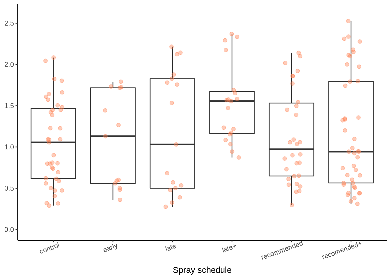

Box plots of the unsprayed control treatments means for both PM severity (top) and crop yield (bottom), indicating within-season variation (A), and trial treatment means for each spray schedule (B).

3.2 Treatment focused summaries

Various factors have been studied in the collated trials which may influence the subsequent meta-analysis. A quick inspection of the following factors were done to examine the possible influence these variables may have on on mungbean grain yield and/or powdery mildew mean plot severity.

Fungicide type (propiconazole and tebuconazole)
1. Fungicide Doses
2. Number of fungicide sprays
3. Host cultivar (probably is a co-variate with season due to changing cultivars over time)
4. Row spacing
5. Final disease rating / disease pressure
6. Moisture availability for the crop

The data plotted below are from 16 field trials between (2011 - 2019) of which the details are described in the Trials considered for inclusion in meta-analysis.

3.2.1 Fungicide type

3.2.1.1 Powdery mildew severity

n_C <- sum(PM_MB_dat$fungicide_ai == "control")
n_P <- sum(PM_MB_dat$fungicide_ai == "propiconazole")
n_T <- sum(PM_MB_dat$fungicide_ai == "tebuconazole")

PM_MB_dat %>%
   ggplot(aes(y = PM_final_severity, x = as.factor(fungicide_ai))) +
   xlab("Fungicide treatment") +
   ggtitle(label = "Powdery mildew severity for each fungicide active ingredient") +
   labs(caption = paste("Control n:", n_C,
                        "; Propiconazole n:", n_P,
                        "; Tebuconazole n:", n_T, sep = "")) +
   geom_boxplot()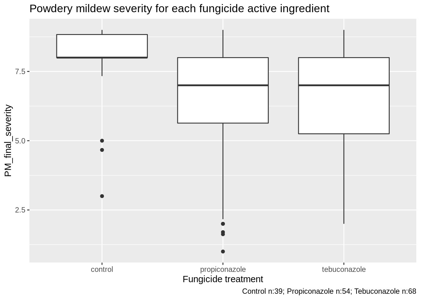

3.2.1.2 Yield effect

PM_MB_dat %>%
   ggplot(aes(y = grain_yield.t.ha., x = as.factor(fungicide_ai))) +
   xlab("Fungicide treatment") +
   ggtitle(label = "Grain yield for each fungicide active ingredient") +
   labs(caption = paste("Control n:", n_C,
                        "; Propiconazole n:", n_P,
                        "; Tebuconazole n:", n_T, sep = "")) +
   geom_boxplot()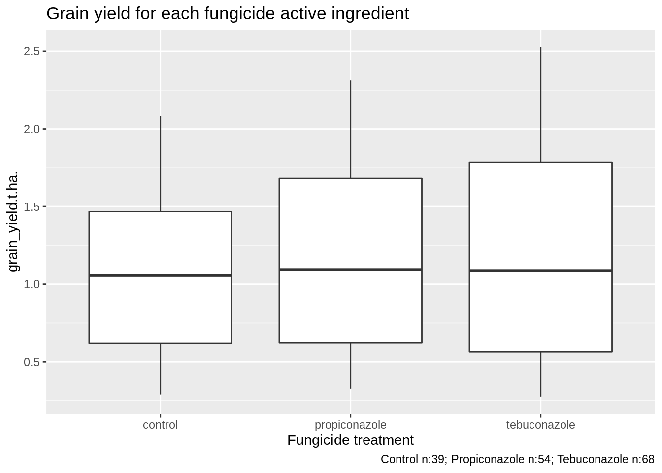

3.2.2 Fungicide Doses

This analysis focuses only the DMI fungicides, tebuconazole and propiconazole, which were trialled the most often.

We should check that all fungicide doses that were used were roughly the same, if we are to compare between trials where dose might be different.

PM_MB_dat %>%
   filter(fungicide_ai == "tebuconazole" |
             fungicide_ai == "propiconazole") %>%
   ggplot(aes(x = as.factor(dose_ai.ha), fill = fungicide_ai)) +
   xlab("Dose (g ai/ha)") +
   ggtitle(label = "Total number of treatments for each respective tebuconazole\nor propiconazole dose") +
   geom_bar()

All trials that used tebuconazole used approximately the same dose. Dose of the active ingredient ranged from 62.35 g per hectare to 60 g per hectare.

Doses for propiconazole range from 62.5 g to 125 g, a large variation.
Let’s inspect the difference in yields for each dose.

PM_MB_dat %>%
   filter(fungicide_ai == "propiconazole") %>%
   ggplot(aes(x = relevel(as.factor(dose_ai.ha), "62.5"), y = grain_yield.t.ha.)) +
   xlab("Dose (g ai/ha)") +
   labs(label = "Yield for each respective propiconazole dose",
        caption = "Facets indicate the number of applications") +
   geom_boxplot(fill = "grey", alpha = 0.5) +
   ylab("Grain yield t / ha") +
   facet_grid(cols = vars(total_fungicide))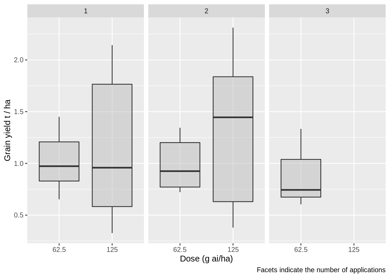

This dose effect should be investigated in the meta-analysis.

How many treatments of each dose have been investigated per trial?

table(as.character(PM_MB_dat[PM_MB_dat$fungicide_ai == "propiconazole",]$trial_ref),
      PM_MB_dat[PM_MB_dat$fungicide_ai == "propiconazole",]$dose_ai.ha)

##              
##               62.5 125
##   AM1303         3   0
##   AM1304         1   0
##   AM1305         3   0
##   BB1305         3   0
##   mung1112/01    2   2
##   mung1112/02    2   2
##   mung1617/01    0  15
##   mung1617/02    0  15
##   mung1718/01    0   6

3.2.3 Number of fungicide sprays

Inspect the frequency of sprays per fungicide.

table(PM_MB_dat$fungicide_ai, PM_MB_dat$total_fungicide)

##                
##                  0  1  2  3
##   control       39  0  0  0
##   propiconazole  0 26 25  3
##   tebuconazole   0 34 32  2

Very few treatments were sprayed more than three times and only in AM1305, AM1303, BB1305, mung1516/01, mung1516/02

3.2.4 Mungbean cultivars

Australian mungbean varieties have the following resistance to powdery mildew.

Berken: Highly susceptible
- Crystal: Susceptible
- Jade: Moderately susceptible

Let’s view a stacked bar plot of the number of sprays for both demethylation inhibitors, tebuconazole and propiconazole against each cultivar.

PM_MB_dat %>%
   filter(fungicide_ai == "tebuconazole" |
             fungicide_ai == "propiconazole") %>%
   group_by(host_genotype, fungicide_ai, trial_ref) %>%
   summarise() %>%
   count() %>%
   rename(Treatments = n) %>%
   ggplot(aes(x = host_genotype, y = Treatments, fill = fungicide_ai)) +
   xlab("Cultivar") +
   ylab("N Trials") +
   ggtitle(label = "Cultivars used in either tebuconazole or propiconazole trials") +
   geom_col() +
   scale_fill_discrete(name = "Fungicide AI")

3.2.4.1 Yield loss in cultivar Jade

Cultivar Jade shows the best quantitative resistance to powdery mildew. Based on the 2016 GRDC report by Sue Thompson (2016) we want to know what is the possible yield loss for this moderately susceptible cultivar.

PM_MB_dat %>%
   filter(year == "2016",
          host_genotype == "Jade") %>%
   mutate(
      Treatment = case_when(
         fungicide_ai == "control" ~ "control_yield",
         TRUE ~ "FungicideTreated_yield"
      )
   ) %>%
   group_by(location, Treatment) %>%
   summarise(
      trial_ref = trial_ref,
      location = location,
      year = year,
      Yield = mean(grain_yield.t.ha., na.rm = TRUE),
      .groups = "drop"
   ) %>%
   distinct() %>%
   pivot_wider(names_from = Treatment, values_from = Yield) %>%
   mutate(Diff = FungicideTreated_yield - control_yield) %>%
   mutate(percent = (Diff / FungicideTreated_yield) * 100) %>%
   dplyr::select(trial_ref,
                 location,
                 year,
                 control_yield,
                 FungicideTreated_yield,
                 percent,
                 Diff) %>%
   flextable()

trial_ref	location	year	control_yield	FungicideTreated_yield	percent	Diff
mung1516/01	Hermitage	2016	1.8029	2.2821833	21.00109	0.4792833
mung1516/02	Kingaroy	2016	0.8107	0.9541167	15.03136	0.1434167

3.2.5 Row spacing

Some experiments were designed to investigate the effect of row spacing and plant density on powdery mildew disease as well as fungicide timing and efficacy. The results showed that the row spacing had no statistically significant effect on powdery mildew, but narrower rows in most cases increased yield significantly. This finding has also been shown by several other researchers’ work in Queensland and New South Wales as well.

PM_MB_dat %>%
   filter(fungicide_ai == "tebuconazole" |
             fungicide_ai == "propiconazole") %>%
   group_by(fungicide_ai, row_spacing, trial_ref) %>%
   summarise() %>%
   count() %>%
   rename(Trials = n) %>%
   ggplot(aes(x = as.factor(row_spacing), y = Trials)) +
   xlab("Row Spacing (m)") +
   ylab("N Trials") +
   ggtitle(label = "Trial row spacing using tebuconazole") +
   geom_col(aes(fill = fungicide_ai),
            position = "dodge") +
   scale_fill_discrete(name = "Fungicide AI")

## `summarise()` has grouped output by 'fungicide_ai', 'row_spacing'. You can override using the `.groups` argument.

Will plotting row spacing treatments show differences for the response variables, yield and disease severity. The main questions are: * Were there any statistical differences for mungbean yield or powdery mildew severity between row spacing treatments? * If not, can we pool certain row spacing that have no significant difference?

# Which row spacing leads to the higher disease severity
PM_MB_dat %>%
   filter(year == 2017 |
             year == 2018) %>%
   filter(fungicide_ai == "control") %>%
   ggplot(aes(y = PM_final_severity, x = factor(row_spacing))) +
   geom_boxplot(alpha = 0.5) +
   ylab("Final severity rating") +
   xlab("Row spacing (m)") +
   ggtitle("Powdery mildew severity between different row spacing across all trials")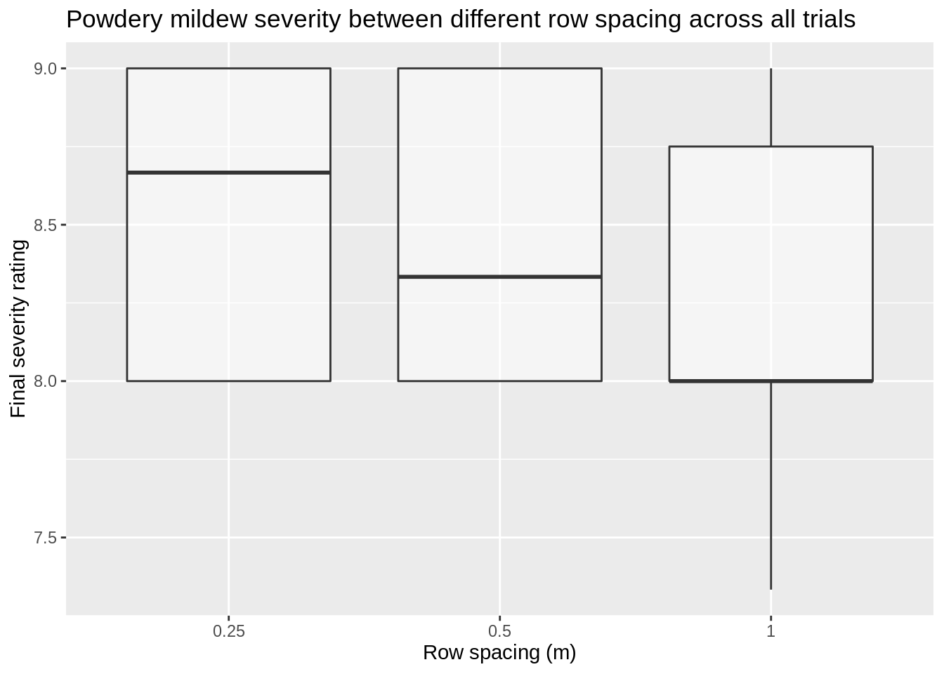

There is little difference here between the row spacing treatments, Let’s look if there is a trial location effect as disease pressure lead to varying results.

# Does trial year and location interact between row spacing and disease severity
PM_MB_dat %>%
   filter(year == 2017 |
             year == 2018) %>%
   filter(fungicide_ai == "control") %>%
   ggplot(aes(y = PM_final_severity, x = factor(row_spacing))) +
   geom_boxplot(alpha = 0.5) +
   facet_grid(cols = vars(location)) +
   ggtitle("Powdery mildew variation between different row spacing") +
   ylab("Final severity rating") +
   xlab("Row spacing (m)")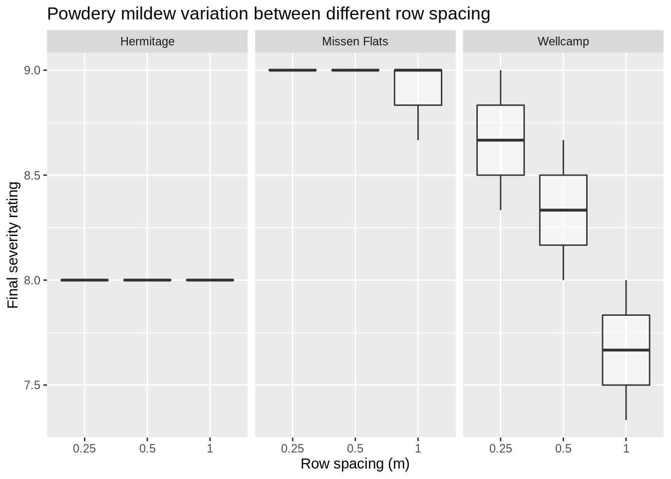

In the Wellcamp site, wider row spacing reduces PM severity, the other sites it seems there was not enough variation to make a distinction between row spacing treatments.

# Which row spacing leads to the higher yield potential
PM_MB_dat %>%
   filter(year == 2017 |
             year == 2018) %>%
   ggplot(aes(
      y = as.numeric(grain_yield.t.ha.),
      x = as.factor(row_spacing),
      colour = location
   )) +
   geom_jitter(width = 0.05) +
   ggtitle("Grain yield results for different row spacing at three locations") +
   xlab("Row spacing (m)") +
   ylab("Grain yield (t/ha)")+
   theme_classic()

The plots seem to imply when yield is limited, presumably by other abiotic factors, there is no effect of row spacing on yield, like in the Hermitage trial. However, if the average yield is more than approximately 1 t/ha then smaller row spacing has the potential to provide greater yield per hectare.

Overall row spacing may influence both powdery mildew severity and yield. However, in the trial reports, no significant interaction was found between row spacing, powdery mildew severity and yield. That is, with narrower row spacing appeared to increase yield even if the amount of powdery mildew increased and no relationship could be detected between an interaction of the three.

3.2.6 Disease pressure

The amount of disease pressure between seasons is another variable which could impact mungbean yield meta-analysis effect size.

# Assess the effect of yield pressure on the spray schedule efficacy
# Use quantiles to separate disease pressure into High, Medium and low disease pressure categories
DP33 <- 
   PM_MB_dat %>%
   filter(fungicide_ai == "control") %>%
   pull(PM_final_severity) %>%
   quantile(0.3333)

DP66 <- 
   PM_MB_dat %>%
   filter(fungicide_ai == "control") %>%
   pull(PM_final_severity) %>%
   quantile(0.6666)

PM_MB_dat %>%
   mutate(yc = case_when(fungicide_ai == "control" ~ grain_yield.t.ha.,
                         TRUE ~ NA_real_))%>%
   group_by(trial_ref)%>%
   mutate(yc = mean(yc, na.rm=TRUE)) %>%
   mutate(yield_saved = case_when(fungicide_ai != "control" ~ grain_yield.t.ha. - yc,
                    fungicide_ai == "control" ~ NA_real_)) %>%
   mutate(dc = case_when(fungicide_ai == "control" ~ PM_final_severity,
                         TRUE ~ NA_real_))%>%
   mutate(dc = mean(dc, na.rm = TRUE))%>%
   ungroup() %>%
   mutate(disease_pressure = case_when(dc <= DP33 ~ "low",
                                 dc <= DP66 &
                                 dc > DP33 ~ "medium",
                                 dc > DP66 ~ "high",
                                 TRUE ~ NA_character_))%>%
   filter(spray_management != "control") %>%
   ggplot(aes(disease_pressure, yield_saved))+
   geom_boxplot()+ 
   facet_grid(. ~ spray_management)

From these plots it is difficult to determine if there is an interaction between disease pressure and the yield saved, or if no interaction exists and fungicide efficacy in general has greater potential to save yield when disease pressure is higher. It is worth noting there was not sufficient variation in the control plot disease severity to produce a medium disease severity category.

3.2.7 In-crop rainfall

3.2.7.1 Whole season

In season rainfall is known to contribute significantly to crop yields, however the timing of rainfall is likely important.

First an inspection of all rainfall within the season

source("R/add_lat_longs.R") # code adds the latitude- and longitude to PM_MB_dat
source("R/crop_rain.R")

# Obtain rainfall from bomrang
PM_MB_dat$sum_rain <-
   crop_rain(location_name = PM_MB_dat$location,
          latitude = PM_MB_dat$lat,
          longitude = PM_MB_dat$lon,
          first_day = PM_MB_dat$planting_date,
          last_day = PM_MB_dat$harvest_date)

# Due to the Bureau of Meteorology in Australia blocking requests using the 
#  R package `bomrang` this code has been changed to import the cached values

# plot yield vs rainfall
PM_MB_dat %>%
   ggplot(aes(y = grain_yield.t.ha., x = sum_rain)) + 
   geom_point()

## Warning: Removed 20 rows containing missing values (geom_point).

summary(lm(grain_yield.t.ha. ~ sum_rain, data = PM_MB_dat))

## 
## Call:
## lm(formula = grain_yield.t.ha. ~ sum_rain, data = PM_MB_dat)
## 
## Residuals:
##      Min       1Q   Median       3Q      Max 
## -1.19469 -0.55873 -0.03576  0.57633  1.37833 
## 
## Coefficients:
##               Estimate Std. Error t value Pr(>|t|)    
## (Intercept)  1.6762255  0.2009508   8.341 6.49e-14 ***
## sum_rain    -0.0017944  0.0007276  -2.466   0.0149 *  
## ---
## Signif. codes:  0 '***' 0.001 '**' 0.01 '*' 0.05 '.' 0.1 ' ' 1
## 
## Residual standard error: 0.6295 on 139 degrees of freedom
##   (20 observations deleted due to missingness)
## Multiple R-squared:  0.04192,    Adjusted R-squared:  0.03502 
## F-statistic: 6.081 on 1 and 139 DF,  p-value: 0.01488

3.2.7.2 Early-season rainfall

Here we only look at the effect of rainfall between the planting date and first sign of disease. We are choosing first sign of disease as a mid point in the crop maturity.

PM_MB_dat$early_rain <-
   crop_rain(location_name = PM_MB_dat$location,
          latitude = PM_MB_dat$lat,
          longitude = PM_MB_dat$lon,
          first_day = PM_MB_dat$planting_date,
          last_day = PM_MB_dat$first_sign_disease)

PM_MB_dat %>%
   ggplot(aes(y = grain_yield.t.ha., x = early_rain)) + 
   geom_point()

summary(lm(grain_yield.t.ha. ~ early_rain, data = PM_MB_dat))

## 
## Call:
## lm(formula = grain_yield.t.ha. ~ early_rain, data = PM_MB_dat)
## 
## Residuals:
##      Min       1Q   Median       3Q      Max 
## -1.02549 -0.54188  0.01965  0.52195  1.18905 
## 
## Coefficients:
##               Estimate Std. Error t value Pr(>|t|)    
## (Intercept)  1.6187927  0.1084723  14.924  < 2e-16 ***
## early_rain  -0.0033201  0.0007248  -4.581 9.31e-06 ***
## ---
## Signif. codes:  0 '***' 0.001 '**' 0.01 '*' 0.05 '.' 0.1 ' ' 1
## 
## Residual standard error: 0.573 on 159 degrees of freedom
## Multiple R-squared:  0.1166, Adjusted R-squared:  0.111 
## F-statistic: 20.98 on 1 and 159 DF,  p-value: 9.308e-06

There is a significant negative association here, indicating rain fall early in the crop development negatively affects mungbean yields. However the very low R-squared value indicates it is no a strong one.

3.2.7.3 Late-season rainfall

Here we only look at the effect of rainfall between the first sign of disease and crop harvest.

PM_MB_dat$late_rain <-
   crop_rain(location_name = PM_MB_dat$location,
          latitude = PM_MB_dat$lat,
          longitude = PM_MB_dat$lon,
          first_day = PM_MB_dat$first_sign_disease,
          last_day = PM_MB_dat$harvest_date)


PM_MB_dat %>%
   ggplot(aes(y = grain_yield.t.ha., x = late_rain)) + 
   geom_point()

## Warning: Removed 20 rows containing missing values (geom_point).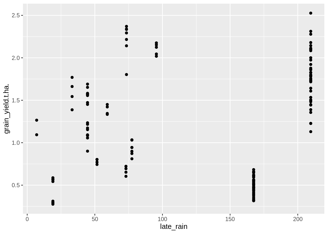

summary(lm(grain_yield.t.ha. ~ late_rain, data = PM_MB_dat))

## 
## Call:
## lm(formula = grain_yield.t.ha. ~ late_rain, data = PM_MB_dat)
## 
## Residuals:
##      Min       1Q   Median       3Q      Max 
## -0.92828 -0.64258  0.03875  0.49696  1.23659 
## 
## Coefficients:
##              Estimate Std. Error t value Pr(>|t|)    
## (Intercept) 1.0467776  0.1112158   9.412   <2e-16 ***
## late_rain   0.0011816  0.0007598   1.555    0.122    
## ---
## Signif. codes:  0 '***' 0.001 '**' 0.01 '*' 0.05 '.' 0.1 ' ' 1
## 
## Residual standard error: 0.6376 on 139 degrees of freedom
##   (20 observations deleted due to missingness)
## Multiple R-squared:  0.0171, Adjusted R-squared:  0.01003 
## F-statistic: 2.418 on 1 and 139 DF,  p-value: 0.1222

There is a significant positive association here, indicating rainfall after disease commences is likely to lead to increased yield. However the very low R-squared value indicates it is no a strong one.

3.2.7.4 Mid-season rainfall

Here we only look at the effect of rainfall between the 20 days after planting and 80 days after planting.

PM_MB_dat$mid_rain <-
   crop_rain(location_name = PM_MB_dat$location,
          latitude = PM_MB_dat$lat,
          longitude = PM_MB_dat$lon,
          first_day = ymd(PM_MB_dat$planting_date) + days(45),
          last_day = ymd(PM_MB_dat$planting_date) + days(75)
   )

PM_MB_dat %>%
   ggplot(aes(y = grain_yield.t.ha., x = mid_rain)) + 
   geom_point()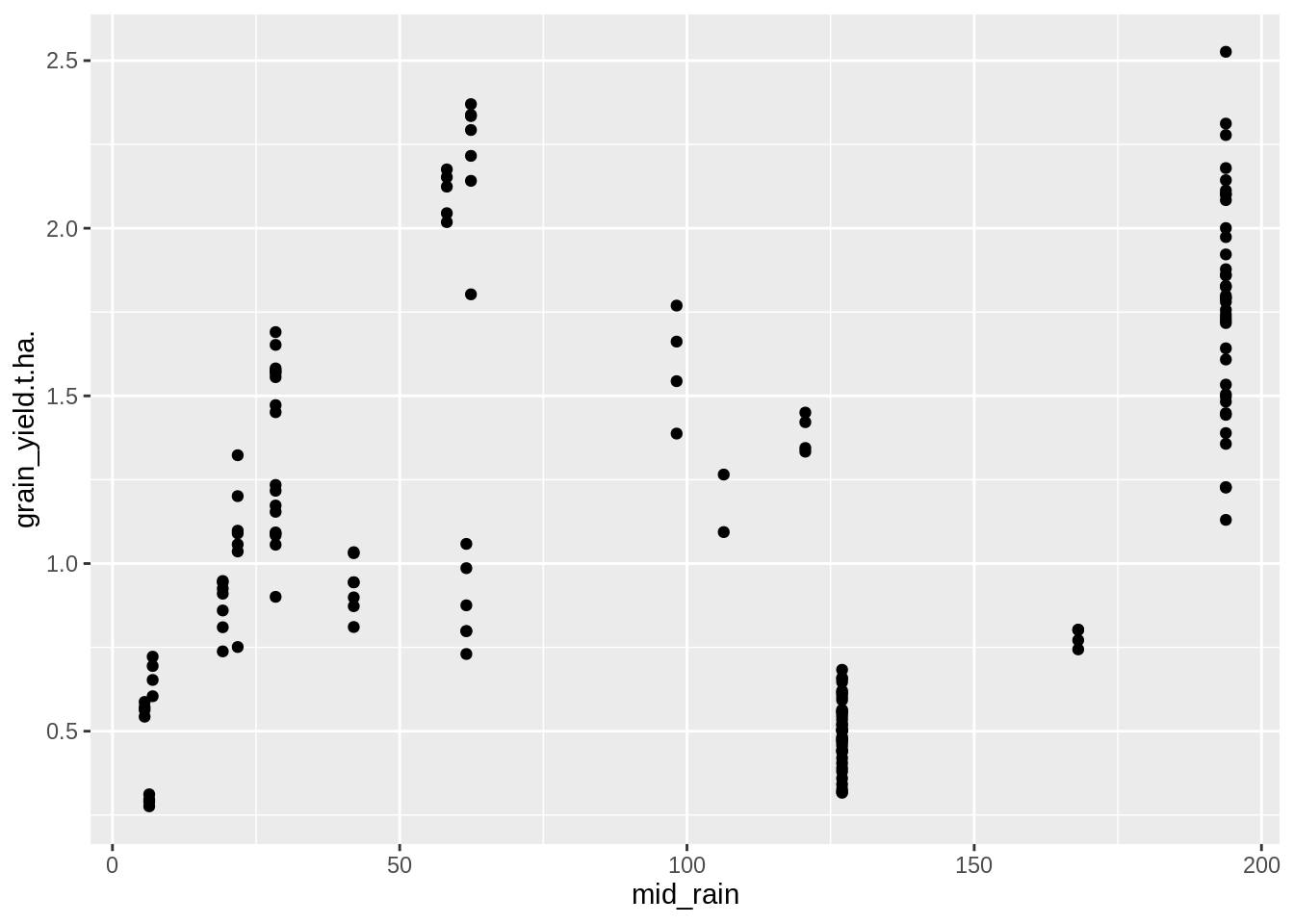

summary(lm(grain_yield.t.ha. ~ mid_rain, data = PM_MB_dat))

## 
## Call:
## lm(formula = grain_yield.t.ha. ~ mid_rain, data = PM_MB_dat)
## 
## Residuals:
##      Min       1Q   Median       3Q      Max 
## -0.91273 -0.58233 -0.00342  0.39919  1.30604 
## 
## Coefficients:
##              Estimate Std. Error t value Pr(>|t|)    
## (Intercept) 0.9047111  0.0841268  10.754  < 2e-16 ***
## mid_rain    0.0025537  0.0006853   3.726 0.000269 ***
## ---
## Signif. codes:  0 '***' 0.001 '**' 0.01 '*' 0.05 '.' 0.1 ' ' 1
## 
## Residual standard error: 0.5846 on 159 degrees of freedom
## Multiple R-squared:  0.08032,    Adjusted R-squared:  0.07454 
## F-statistic: 13.89 on 1 and 159 DF,  p-value: 0.0002694

There is no association with mid season rain and crop yields.

From the plots shown here we can draw the conclusion that we lack sufficient information. Most likely available soil water between trials along with other unobserved variables influence of rainfall on mungbean crops and therefore we will not investigate any further.

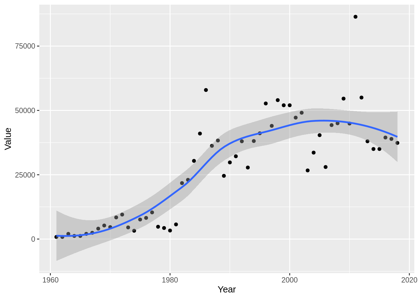
3.2.8 FAO mungbean data

An important consideration for why to carry out work on mungbean diseases is the value the crop provides. Let’s pull in data from the FAOSTAT website for the area of mungbean crops harvested.

beans <- read.csv(here("data/FAOSTAT_data_7-6-2020.csv"))

str(beans)

## 'data.frame':    473 obs. of  15 variables:
##  $ Domain.Code     : chr  "QC" "QC" "QC" "QC" ...
##  $ Domain          : chr  "Crops" "Crops" "Crops" "Crops" ...
##  $ Area.Code       : int  10 10 10 10 10 10 10 10 10 10 ...
##  $ Area            : chr  "Australia" "Australia" "Australia" "Australia" ...
##  $ Element.Code    : int  5312 5419 5510 5312 5419 5510 5312 5419 5510 5312 ...
##  $ Element         : chr  "Area harvested" "Yield" "Production" "Area harvested" ...
##  $ Item.Code       : int  176 176 176 176 176 176 176 176 176 176 ...
##  $ Item            : chr  "Beans, dry" "Beans, dry" "Beans, dry" "Beans, dry" ...
##  $ Year.Code       : int  1961 1961 1961 1962 1962 1962 1963 1963 1963 1964 ...
##  $ Year            : int  1961 1961 1961 1962 1962 1962 1963 1963 1963 1964 ...
##  $ Unit            : chr  "ha" "hg/ha" "tonnes" "ha" ...
##  $ Value           : int  809 5525 447 809 11001 890 2023 5151 1042 1214 ...
##  $ Flag            : chr  "" "Fc" "" "" ...
##  $ Flag.Description: chr  "Official data" "Calculated data" "Official data" "Official data" ...
##  $ Note            : logi  NA NA NA NA NA NA ...

beans %>%
   filter(Item == "Beans, dry",
          Element == "Area harvested") %>%
   dplyr::select(Year, Value) %>%
   ggplot(aes(y = Value, x = Year)) +
   geom_point() +
   geom_smooth()

## `geom_smooth()` using method = 'loess' and formula 'y ~ x'

2 Trials considered for inclusion in meta-analysis

4 Grain yield meta-analysis