5 Powdery mildew severity meta-analysis

An additional question to our main aim: does spray schedule have a similar effect on disease severity?

This model will be similar to the grain yield meta-analysis and use the main variables:

Powdery mildew severity, the response variable (1-9 scale)
- Trial, which resolves combinations of categorical random variables:
  1. year
  2. location
  3. row spacing
  4. cultivar
- spray_management, a moderator to evaluate the difference in effect size attributed to fungicide application timing.
- id, random variable indicating each treatment is independent

Load libraries and data.

if (!require("pacman"))
   install.packages("pacman")
pacman::p_load(tidyverse,
               kableExtra,
               RColorBrewer,
               metafor,
               here,
               netmeta,
               multcomp,
               dplyr,
               flextable,
               gam,
               clubSandwich)

source(here("R/reportP.R"))

# Data
PM_dat_D <-
   read.csv("cache/PM_disease_clean_data.csv", stringsAsFactors = FALSE)

# functions
logit <- function(x){
   log((x)/(1 - x))
}

inv_logit <- function(x){
   exp(x)/(1 + exp(x))
}

5.0.1 Define Trial

PM_dat_D <-
   PM_dat_D %>%
   mutate(trial = paste(trial_ref,
                        year,
                        location,
                        host_genotype,
                        row_spacing,
                        sep = "_"))

5.0.2 Inspect PM severity for normality

Given the meta-analysis assumes powdery mildew severity observations to be a univariate normal distribution \(Y_i = N(\mu , \sigma)\), with a mean \(\mu\) and standard deviation \(\sigma\). We need to inspect severity for a normality.

hist(PM_dat_D$PM_final_severity)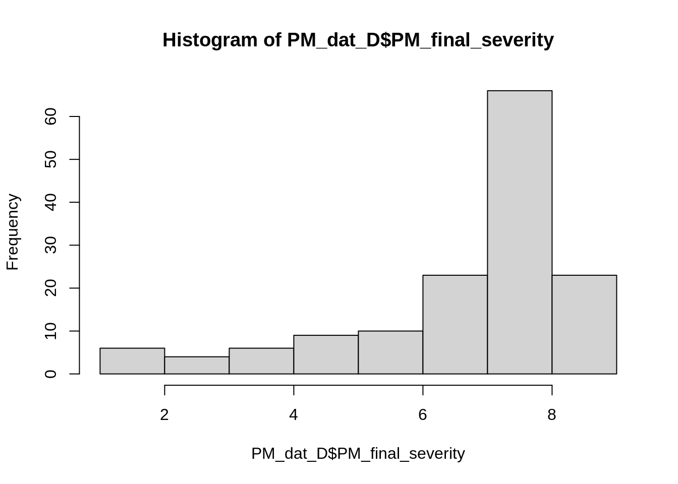

summary(PM_dat_D$PM_final_severity)

##    Min. 1st Qu.  Median    Mean 3rd Qu.    Max. 
##   1.000   6.367   7.667   6.933   8.000   9.000

We can see here that powdery mildew severity observations are skewed towards the top of the scale, eight and nine in this case.

We can improve the normality by transforming the effect size, disease severity, by squaring.

PM_dat_D$yi_square <- PM_dat_D$PM_final_severity ^2
PM_dat_D$vi_square <- (PM_dat_D$vi +1)^2
# Note: Here I added 1 to the variance before it was squared. This is because squaring numbers below one makes the number smaller or remain zero. This does not change the meta-analysis mean estimates but does increase heterogeneity and tao._  

hist(PM_dat_D$yi_square)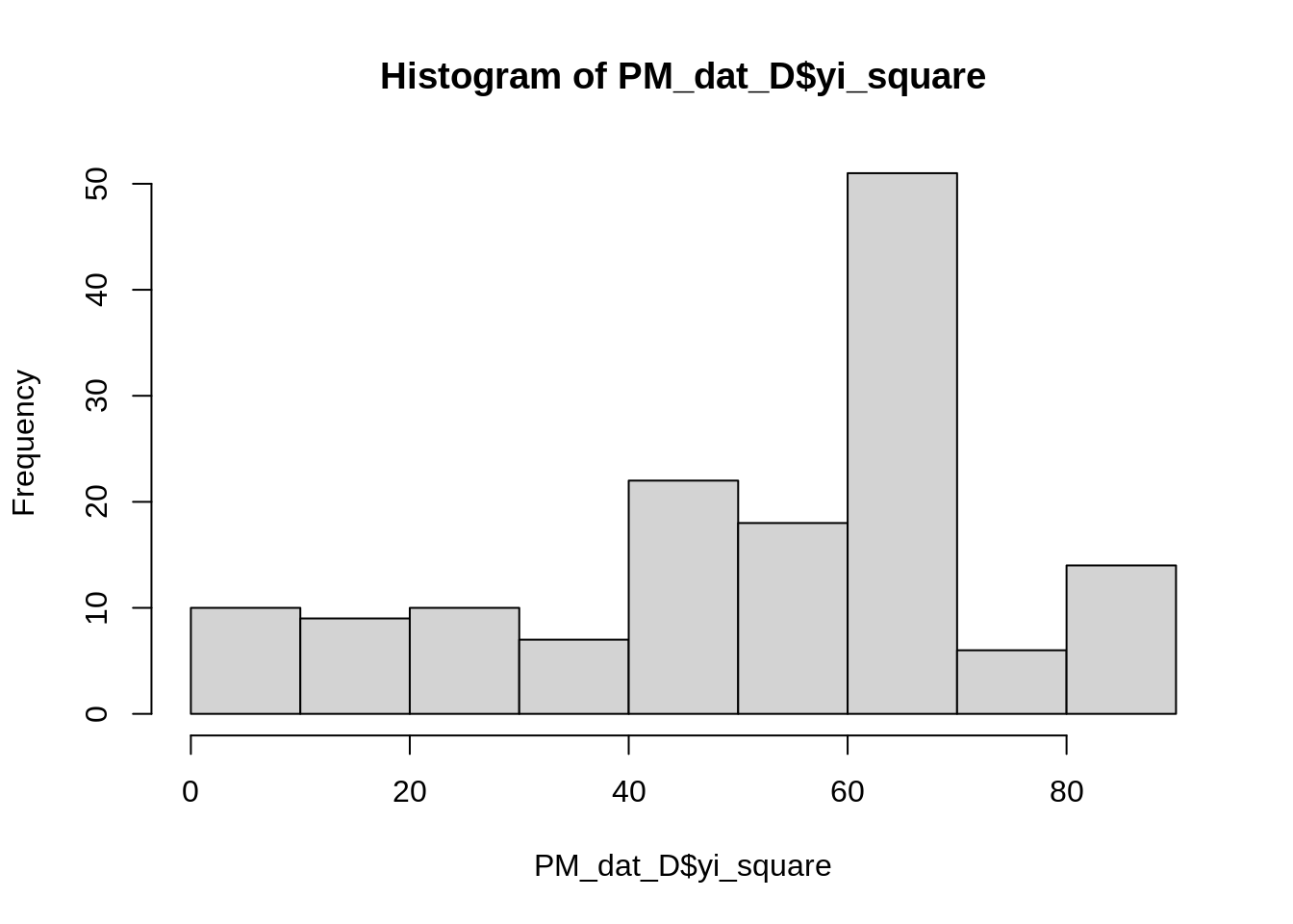

summary(PM_dat_D$yi_square)

##    Min. 1st Qu.  Median    Mean 3rd Qu.    Max. 
##    1.00   40.54   58.78   51.62   64.00   81.00

Another transformation which might be more suitable for a discrete response is either a log() or logit() transformation. However, first we should convert the scale from 1 - 9 to between 0 and 1.

5.0.3 Transform severity response

Let us also transform the severity onto a percentage scale so we can compare the results of meta-analyses with no transformation, squared severity, and percent severity.

This conversion from ordinal scale to a severity rating is described in Table 2 of the paper.

# Percent severity conversion
# define ordinal conversion from scale to proportion
s1 <- 0
s2 <- 0.33 * 0.5
s3 <- 0.5 * 0.87
s4 <- 0.66 * 0.75
s5 <- 0.66 * 0.87
s6 <- 0.66 * 1
s7 <- 0.75 * 1
s8 <- 1 * 0.87
s9 <- 1
x <- c(s1, s2, s3, s4, s5, s6, s7, s8, s9)
y <- c(1:9)
a = data.frame(x, y)
plot(a)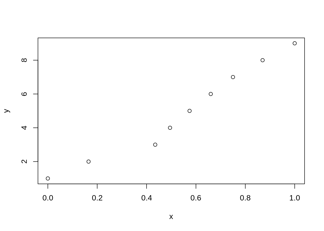

We can fit a GAM curve between the 1 - 9 scale and the new scale between 0 and 1.

# fit a curve using a gam with spline value 0.01
g1 <- gam(x ~ s(y, spar = 0.1), family = gaussian)

# View plot of gam
plot(x = predict(g1,
                 data.frame(y = seq(1, 9, by = 0.1))), y = seq(1, 9, by = 0.1))
points(x, y, col = "red", pch = 16)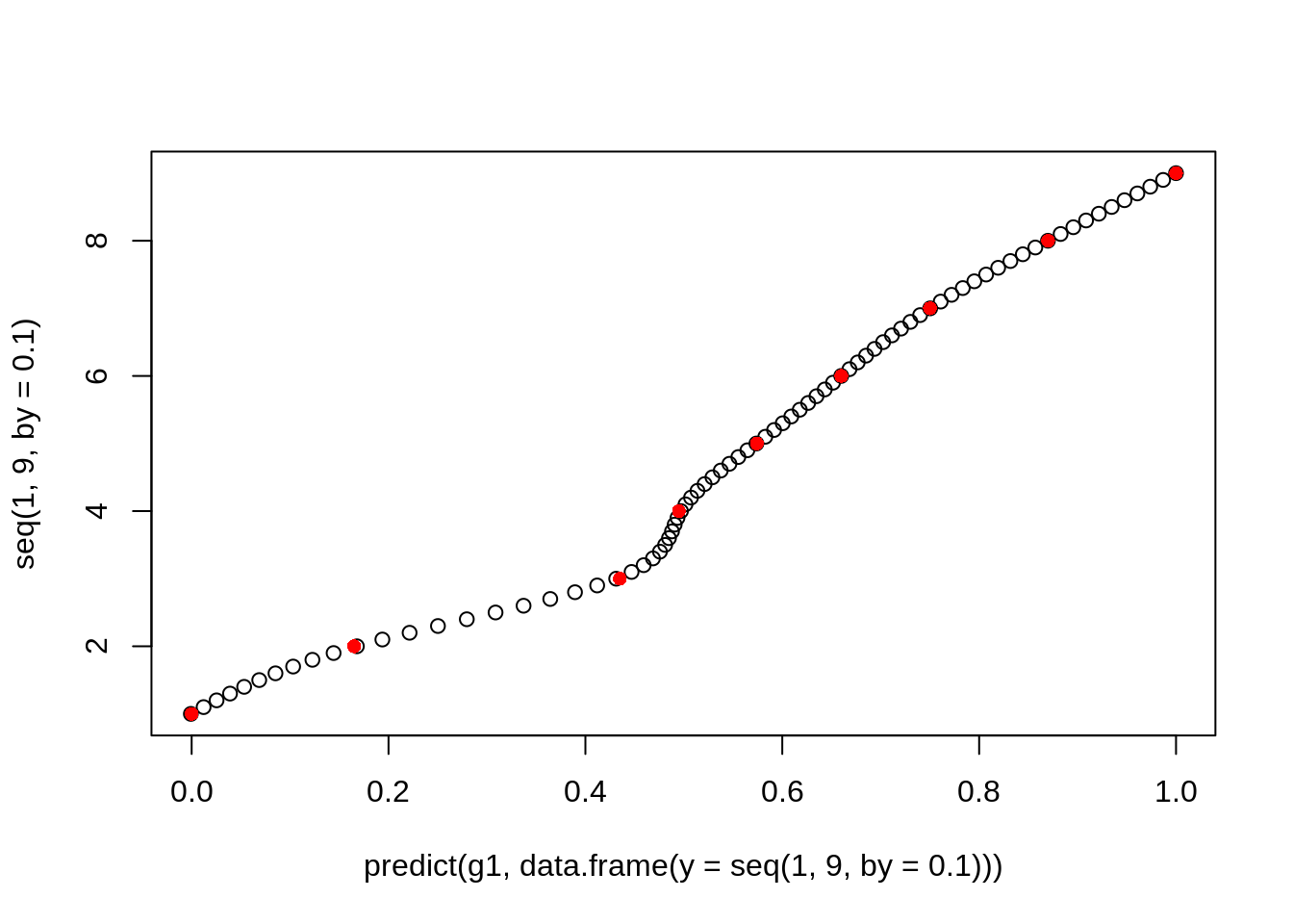

# predict values for dataset
new_sev <- predict(object =  g1,
                   newdata = data.frame(y = PM_dat_D[, "PM_final_severity"]))
# Check fit
plot(x = new_sev, y = PM_dat_D[, "PM_final_severity"])
points(x, y, col = "red", pch = 16)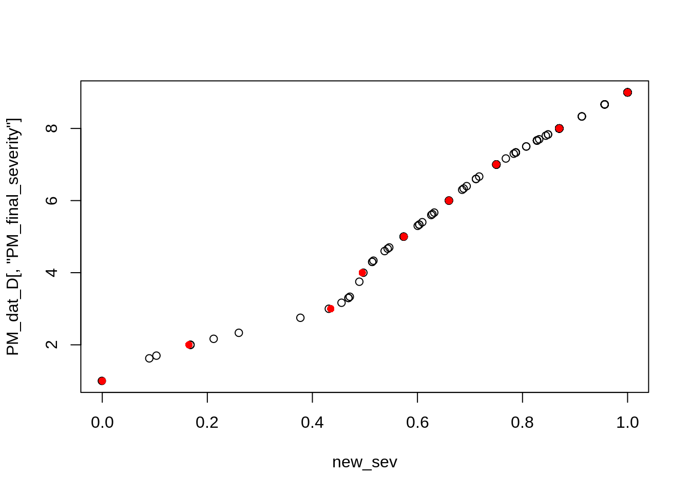

# Allocate new variable percent severity
PM_dat_D$yi_percent <- new_sev

# Conversion of variance
# Here I add the variance and mean severity and predict the conversion value
# then subtract the mean severity to obtain the difference as the sample variance
PM_dat_D$vi_percent  <- predict(object =  g1,
                                newdata = data.frame(y = PM_dat_D[, "vi"] + PM_dat_D[, "PM_final_severity"])) - PM_dat_D$yi_percent


# create log transformed values
PM_dat_D$yi_log <- log(PM_dat_D$yi_percent)

## Warning in log(PM_dat_D$yi_percent): NaNs produced

PM_dat_D$vi_log <-
   (PM_dat_D$vi_percent) / (PM_dat_D$replicates * PM_dat_D$yi_percent ^ 2)

# Correct Inf to 0
PM_dat_D[is.na(PM_dat_D$yi_log), "yi_log"] <- 0
PM_dat_D[PM_dat_D$vi_log == -Inf, "vi_log"] <- 0.001

#logit transformed percentages
PM_dat_D$yi_logit <- logit(PM_dat_D$yi_percent)

## Warning in log((x)/(1 - x)): NaNs produced

# logit transformed variance
PM_dat_D$vi_logit <-
   (PM_dat_D$vi_percent) /
   (PM_dat_D$yi_percent * (1 - PM_dat_D$yi_percent)) ^ 2

# Correct -Inf to zeros
PM_dat_D[is.na(PM_dat_D$yi_logit), "yi_logit"] <- 0

5.1 Disease severity spray schedule meta-analysis

First let’s look at the results of the meta-analysis without transformation

PMsev_mv <- rma.mv(
   yi = PM_final_severity,
   vi,
   mods = ~ spray_management,
   method = "ML",
   random = list(~ spray_management | trial, ~ 1 | id),
   struct = "UN",
   #control = list(optimizer = "optim"),
   data = PM_dat_D
)

## Warning: There are outcomes with non-positive sampling variances.

## Warning: 'V' appears to be not positive definite.

## Warning: Some combinations of the levels of the inner factor never occurred.
## Corresponding rho value(s) fixed to 0.

summary(PMsev_mv)

## 
## Multivariate Meta-Analysis Model (k = 147; method: ML)
## 
##    logLik   Deviance        AIC        BIC       AICc 
## -145.7909        Inf   345.5818   426.3235   358.2877   
## 
## Variance Components:
## 
##             estim    sqrt  nlvls  fixed  factor 
## sigma^2    0.0369  0.1922    147     no      id 
## 
## outer factor: trial            (nlvls = 22)
## inner factor: spray_management (nlvls = 6)
## 
##             estim    sqrt  k.lvl  fixed             level 
## tau^2.1    1.5788  1.2565     37     no           control 
## tau^2.2    2.9285  1.7113     13     no             Early 
## tau^2.3    0.6798  0.8245     15     no              Late 
## tau^2.4    0.0619  0.2488     13     no         Late_plus 
## tau^2.5    4.2455  2.0605     28     no       Recommended 
## tau^2.6    6.9310  2.6327     41     no  Recommended_plus 
## 
##                   rho.cntr  rho.Erly  rho.Late  rho.Lt_p  rho.Rcmm  rho.Rcm_ 
## control                  1    0.8287    0.9646    0.9977    0.9402    0.5966   
## Early               0.8287         1    0.9341    0.0000    0.8077    0.9436   
## Late                0.9646    0.9341         1    0.9720    0.8830    0.7691   
## Late_plus           0.9977    0.0000    0.9720         1    0.9537    0.6407   
## Recommended         0.9402    0.8077    0.8830    0.9537         1    0.6002   
## Recommended_plus    0.5966    0.9436    0.7691    0.6407    0.6002         1   
##                   cntr  Erly  Late  Lt_p  Rcmm  Rcm_ 
## control              -    no    no    no    no    no 
## Early                7     -    no   yes    no    no 
## Late                 9     6     -    no    no    no 
## Late_plus            4     0     1     -    no    no 
## Recommended         18     6     9     1     -    no 
## Recommended_plus    16     6     9     1    16     - 
## 
## Test of Moderators (coefficients 2:6):
## QM(df = 5) = 163.0624, p-val < .0001
## 
## Model Results:
## 
##                                   estimate      se     zval    pval    ci.lb 
## intrcpt                             7.6729  0.2766  27.7415  <.0001   7.1308 
## spray_managementEarly              -1.0439  0.2582  -4.0434  <.0001  -1.5500 
## spray_managementLate               -0.7455  0.1360  -5.4832  <.0001  -1.0120 
## spray_managementLate_plus          -1.3633  0.2383  -5.7207  <.0001  -1.8304 
## spray_managementRecommended        -1.1069  0.2595  -4.2659  <.0001  -1.6155 
## spray_managementRecommended_plus   -3.2476  0.5445  -5.9645  <.0001  -4.3148 
##                                     ci.ub 
## intrcpt                            8.2150  *** 
## spray_managementEarly             -0.5379  *** 
## spray_managementLate              -0.4790  *** 
## spray_managementLate_plus         -0.8962  *** 
## spray_managementRecommended       -0.5983  *** 
## spray_managementRecommended_plus  -2.1804  *** 
## 
## ---
## Signif. codes:  0 '***' 0.001 '**' 0.01 '*' 0.05 '.' 0.1 ' ' 1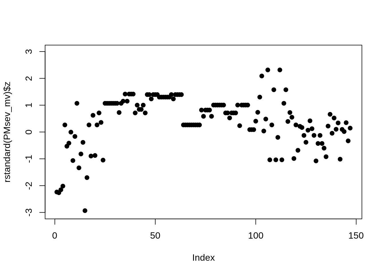

plot(rstandard(PMsev_mv)$z, ylim = c(-3, 3), pch = 19)

This analysis shows the residual are slightly unbalanced and perhaps an effect of time. Does squaring the response improve the residuals?

PMsev_mvSQ <- rma.mv(
   yi = yi_square,
   V = vi_square,
   mods = ~ spray_management,
   method = "ML",
   random = list(~ spray_management | trial, ~ 1 | id),
   struct = "UN",
   control = list(optimizer = "optim"),
   data = PM_dat_D
)

## Warning: Some combinations of the levels of the inner factor never occurred.
## Corresponding rho value(s) fixed to 0.

summary(PMsev_mvSQ)

## 
## Multivariate Meta-Analysis Model (k = 147; method: ML)
## 
##    logLik   Deviance        AIC        BIC       AICc 
## -532.3560   726.4536  1118.7120  1199.4537  1131.4179   
## 
## Variance Components:
## 
##              estim    sqrt  nlvls  fixed  factor 
## sigma^2    23.3194  4.8290    147     no      id 
## 
## outer factor: trial            (nlvls = 22)
## inner factor: spray_management (nlvls = 6)
## 
##               estim     sqrt  k.lvl  fixed             level 
## tau^2.1    306.0169  17.4933     37     no           control 
## tau^2.2    306.3846  17.5038     13     no             Early 
## tau^2.3    134.8188  11.6111     15     no              Late 
## tau^2.4     20.9591   4.5781     13     no         Late_plus 
## tau^2.5    575.9514  23.9990     28     no       Recommended 
## tau^2.6    891.6918  29.8612     41     no  Recommended_plus 
## 
##                   rho.cntr  rho.Erly  rho.Late  rho.Lt_p  rho.Rcmm  rho.Rcm_ 
## control                  1    0.9817    0.9321    1.0000    0.7906    0.8253   
## Early               0.9817         1    0.9839    0.0000    0.7816    0.9024   
## Late                0.9321    0.9839         1    0.9306    0.7456    0.9440   
## Late_plus           1.0000    0.0000    0.9306         1    0.7904    0.8233   
## Recommended         0.7906    0.7816    0.7456    0.7904         1    0.8436   
## Recommended_plus    0.8253    0.9024    0.9440    0.8233    0.8436         1   
##                   cntr  Erly  Late  Lt_p  Rcmm  Rcm_ 
## control              -    no    no    no    no    no 
## Early                7     -    no   yes    no    no 
## Late                 9     6     -    no    no    no 
## Late_plus            4     0     1     -    no    no 
## Recommended         18     6     9     1     -    no 
## Recommended_plus    16     6     9     1    16     - 
## 
## Test for Residual Heterogeneity:
## QE(df = 141) = 30608.5216, p-val < .0001
## 
## Test of Moderators (coefficients 2:6):
## QM(df = 5) = 140.8577, p-val < .0001
## 
## Model Results:
## 
##                                   estimate      se     zval    pval     ci.lb 
## intrcpt                            60.0043  3.8371  15.6378  <.0001   52.4836 
## spray_managementEarly              -4.0626  1.9081  -2.1292  0.0332   -7.8023 
## spray_managementLate              -11.9164  2.3694  -5.0292  <.0001  -16.5604 
## spray_managementLate_plus         -17.4846  3.2357  -5.4037  <.0001  -23.8264 
## spray_managementRecommended       -17.3870  3.7880  -4.5900  <.0001  -24.8113 
## spray_managementRecommended_plus  -38.1953  4.6263  -8.2561  <.0001  -47.2628 
##                                      ci.ub 
## intrcpt                            67.5249  *** 
## spray_managementEarly              -0.3229    * 
## spray_managementLate               -7.2724  *** 
## spray_managementLate_plus         -11.1428  *** 
## spray_managementRecommended        -9.9626  *** 
## spray_managementRecommended_plus  -29.1278  *** 
## 
## ---
## Signif. codes:  0 '***' 0.001 '**' 0.01 '*' 0.05 '.' 0.1 ' ' 1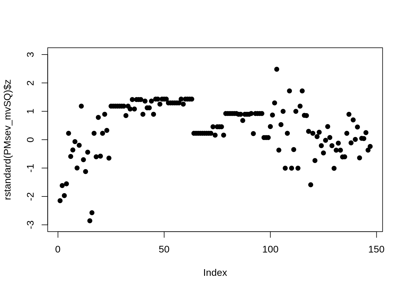

plot(rstandard(PMsev_mvSQ)$z,
     ylim = c(-3, 3),
     pch = 19)

This meta-analysis is more in-line with estimates from the yield meta-analysis. Early sprays are not effective at reducing powdery mildew severity and two or more sprays had higher efficacy than single sprays. Recommended sprays were the most effective spray timing at reducing disease severity.

However square severity is not common when evaluating a response that was obtained on a scale. Log transformed is a more common method of evaluating non-normal disease severity.

Let’s assess the log transformed percent severity.

# remove controls for response ratio meta-analysis
PMsev_mv_log <- rma.mv(
   yi = yi_log,
   V = yi_log,
   mods = ~ spray_management,
   method = "ML",
   random = list(~ spray_management | trial, ~ 1 | id),
   struct = "UN",
   control = list(optimizer = "optim"),
   data = PM_dat_D
)

## Warning: There are outcomes with non-positive sampling variances.

## Warning: Negative sampling variances constrained to zero.

## Warning: 'V' appears to be not positive definite.

## Warning: Some combinations of the levels of the inner factor never occurred.
## Corresponding rho value(s) fixed to 0.

summary(PMsev_mv_log)

## 
## Multivariate Meta-Analysis Model (k = 147; method: ML)
## 
##   logLik  Deviance       AIC       BIC      AICc 
## -23.7322       Inf  101.4645  182.2061  114.1703   
## 
## Variance Components:
## 
##             estim    sqrt  nlvls  fixed  factor 
## sigma^2    0.0497  0.2230    147     no      id 
## 
## outer factor: trial            (nlvls = 22)
## inner factor: spray_management (nlvls = 6)
## 
##             estim    sqrt  k.lvl  fixed             level 
## tau^2.1    0.0207  0.1438     37     no           control 
## tau^2.2    0.0666  0.2580     13     no             Early 
## tau^2.3    0.0105  0.1026     15     no              Late 
## tau^2.4    0.0000  0.0067     13     no         Late_plus 
## tau^2.5    0.1564  0.3954     28     no       Recommended 
## tau^2.6    0.2733  0.5228     41     no  Recommended_plus 
## 
##                   rho.cntr  rho.Erly  rho.Late  rho.Lt_p  rho.Rcmm  rho.Rcm_ 
## control                  1    0.9272    0.9080    0.9951    0.9649    0.8100   
## Early               0.9272         1    0.9988    0.0000    0.7962    0.9707   
## Late                0.9080    0.9988         1    0.8622    0.7661    0.9812   
## Late_plus           0.9951    0.0000    0.8622         1    0.9861    0.7481   
## Recommended         0.9649    0.7962    0.7661    0.9861         1    0.6275   
## Recommended_plus    0.8100    0.9707    0.9812    0.7481    0.6275         1   
##                   cntr  Erly  Late  Lt_p  Rcmm  Rcm_ 
## control              -    no    no    no    no    no 
## Early                7     -    no   yes    no    no 
## Late                 9     6     -    no    no    no 
## Late_plus            4     0     1     -    no    no 
## Recommended         18     6     9     1     -    no 
## Recommended_plus    16     6     9     1    16     - 
## 
## Test of Moderators (coefficients 2:6):
## QM(df = 5) = 32.1577, p-val < .0001
## 
## Model Results:
## 
##                                   estimate      se     zval    pval    ci.lb 
## intrcpt                            -0.1940  0.0481  -4.0353  <.0001  -0.2883 
## spray_managementEarly              -0.1571  0.0822  -1.9111  0.0560  -0.3182 
## spray_managementLate               -0.1017  0.0705  -1.4416  0.1494  -0.2400 
## spray_managementLate_plus          -0.1391  0.0778  -1.7886  0.0737  -0.2915 
## spray_managementRecommended        -0.2561  0.0853  -3.0035  0.0027  -0.4232 
## spray_managementRecommended_plus   -0.5686  0.1165  -4.8810  <.0001  -0.7969 
##                                     ci.ub 
## intrcpt                           -0.0998  *** 
## spray_managementEarly              0.0040    . 
## spray_managementLate               0.0366      
## spray_managementLate_plus          0.0133    . 
## spray_managementRecommended       -0.0890   ** 
## spray_managementRecommended_plus  -0.3403  *** 
## 
## ---
## Signif. codes:  0 '***' 0.001 '**' 0.01 '*' 0.05 '.' 0.1 ' ' 1

plot(rstandard(PMsev_mv_log)$z,
     ylim = c(-3.2, 3),
     pch = 19)

The plot of the residuals show the model is not normally distributed. In addition the estimates don’t reflect what can be observed in the raw data. Log transformed percent severity is therefore no a suitable transformation.

Finally let’s assess the logit transformed percent severity.

# remove controls for response ratio meta-analysis
PMsev_mvPer <- rma.mv(
   yi = yi_logit,
   V = yi_logit,
   mods = ~ spray_management,
   method = "ML",
   random = list(~ spray_management | trial, ~ 1 | id),
   struct = "UN",
   control = list(optimizer = "optim"),
   data = PM_dat_D
)

## Warning: There are outcomes with non-positive sampling variances.

## Warning: Negative sampling variances constrained to zero.

## Warning: 'V' appears to be not positive definite.

## Warning: Some combinations of the levels of the inner factor never occurred.
## Corresponding rho value(s) fixed to 0.

summary(PMsev_mvPer)

## 
## Multivariate Meta-Analysis Model (k = 147; method: ML)
## 
##    logLik   Deviance        AIC        BIC       AICc 
## -254.6073        Inf   563.2146   643.9563   575.9205   
## 
## Variance Components:
## 
##             estim    sqrt  nlvls  fixed  factor 
## sigma^2    0.2978  0.5457    147     no      id 
## 
## outer factor: trial            (nlvls = 22)
## inner factor: spray_management (nlvls = 6)
## 
##             estim    sqrt  k.lvl  fixed             level 
## tau^2.1    4.0250  2.0062     37     no           control 
## tau^2.2    2.9086  1.7054     13     no             Early 
## tau^2.3    0.0918  0.3030     15     no              Late 
## tau^2.4    0.0029  0.0538     13     no         Late_plus 
## tau^2.5    0.9843  0.9921     28     no       Recommended 
## tau^2.6    1.2059  1.0982     41     no  Recommended_plus 
## 
##                   rho.cntr  rho.Erly  rho.Late  rho.Lt_p  rho.Rcmm  rho.Rcm_ 
## control                  1    0.9992    0.9799    0.9995    0.8628    0.8191   
## Early               0.9992         1    0.9869    0.0000    0.8818    0.8407   
## Late                0.9799    0.9869         1    0.9733    0.9463    0.9170   
## Late_plus           0.9995    0.0000    0.9733         1    0.8467    0.8009   
## Recommended         0.8628    0.8818    0.9463    0.8467         1    0.9967   
## Recommended_plus    0.8191    0.8407    0.9170    0.8009    0.9967         1   
##                   cntr  Erly  Late  Lt_p  Rcmm  Rcm_ 
## control              -    no    no    no    no    no 
## Early                7     -    no   yes    no    no 
## Late                 9     6     -    no    no    no 
## Late_plus            4     0     1     -    no    no 
## Recommended         18     6     9     1     -    no 
## Recommended_plus    16     6     9     1    16     - 
## 
## Test of Moderators (coefficients 2:6):
## QM(df = 5) = 45.9481, p-val < .0001
## 
## Model Results:
## 
##                                   estimate      se     zval    pval    ci.lb 
## intrcpt                             2.4499  0.5026   4.8748  <.0001   1.4649 
## spray_managementEarly              -0.4833  0.4791  -1.0089  0.3130  -1.4223 
## spray_managementLate               -1.2147  0.5648  -2.1509  0.0315  -2.3216 
## spray_managementLate_plus          -1.5524  0.5787  -2.6825  0.0073  -2.6866 
## spray_managementRecommended        -1.8393  0.4268  -4.3093  <.0001  -2.6759 
## spray_managementRecommended_plus   -2.5308  0.4183  -6.0501  <.0001  -3.3506 
##                                     ci.ub 
## intrcpt                            3.4349  *** 
## spray_managementEarly              0.4556      
## spray_managementLate              -0.1078    * 
## spray_managementLate_plus         -0.4182   ** 
## spray_managementRecommended       -1.0028  *** 
## spray_managementRecommended_plus  -1.7109  *** 
## 
## ---
## Signif. codes:  0 '***' 0.001 '**' 0.01 '*' 0.05 '.' 0.1 ' ' 1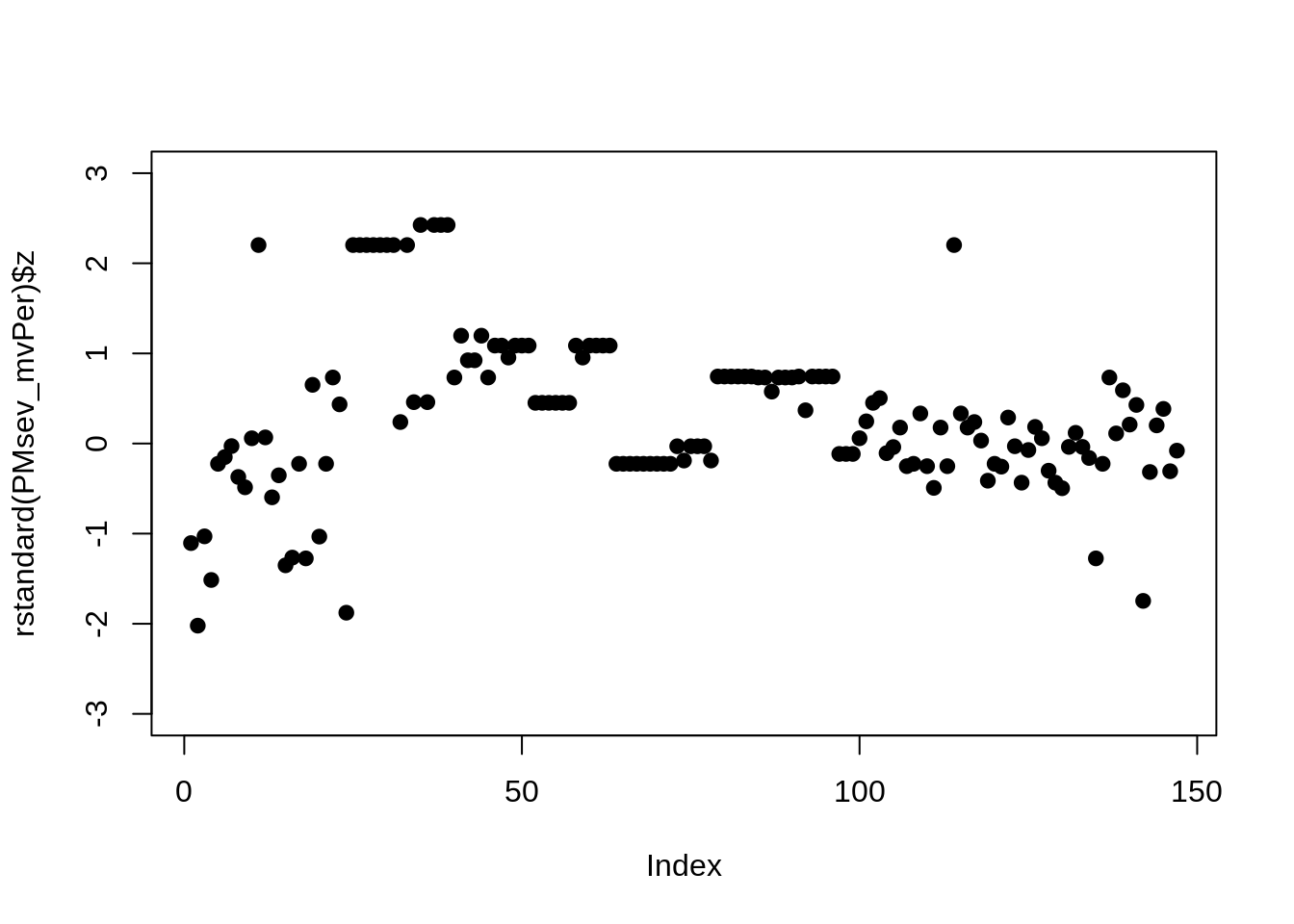

# plot the model residuals
plot(rstandard(PMsev_mvPer)$z,
     ylim = c(-3, 3),
     pch = 19)

s_analysis <-
   lapply(unique(PM_dat_D$trial_ref), function(Trial) {
      dat <- filter(PM_dat_D, trial_ref != Trial)
      # remove controls for response ratio meta-analysis
      rma.mv(
         yi = yi_logit,
         V = yi_logit,
         mods = ~ spray_management,
         method = "ML",
         random = list( ~ spray_management | trial, ~ 1 | id),
         struct = "UN",
         control = list(optimizer = "optim"),
         data = dat
      )
      
   })

## Warning: There are outcomes with non-positive sampling variances.

## Warning: Negative sampling variances constrained to zero.

## Warning: 'V' appears to be not positive definite.

## Warning: Some combinations of the levels of the inner factor never occurred.
## Corresponding rho value(s) fixed to 0.

## Warning: There are outcomes with non-positive sampling variances.

## Warning: Negative sampling variances constrained to zero.

## Warning: 'V' appears to be not positive definite.

## Warning: Some combinations of the levels of the inner factor never occurred.
## Corresponding rho value(s) fixed to 0.

## Warning: There are outcomes with non-positive sampling variances.

## Warning: Negative sampling variances constrained to zero.

## Warning: 'V' appears to be not positive definite.

## Warning: Some combinations of the levels of the inner factor never occurred.
## Corresponding rho value(s) fixed to 0.

## Warning: There are outcomes with non-positive sampling variances.

## Warning: Negative sampling variances constrained to zero.

## Warning: 'V' appears to be not positive definite.

## Warning: Some combinations of the levels of the inner factor never occurred.
## Corresponding rho value(s) fixed to 0.

## Warning: There are outcomes with non-positive sampling variances.

## Warning: Negative sampling variances constrained to zero.

## Warning: 'V' appears to be not positive definite.

## Warning: Some combinations of the levels of the inner factor never occurred.
## Corresponding rho value(s) fixed to 0.

## Warning: There are outcomes with non-positive sampling variances.

## Warning: Negative sampling variances constrained to zero.

## Warning: 'V' appears to be not positive definite.

## Warning: Some combinations of the levels of the inner factor never occurred.
## Corresponding rho value(s) fixed to 0.

## Warning: There are outcomes with non-positive sampling variances.

## Warning: Negative sampling variances constrained to zero.

## Warning: 'V' appears to be not positive definite.

## Warning: Some combinations of the levels of the inner factor never occurred.
## Corresponding rho value(s) fixed to 0.

## Warning: There are outcomes with non-positive sampling variances.

## Warning: Negative sampling variances constrained to zero.

## Warning: 'V' appears to be not positive definite.

## Warning: Some combinations of the levels of the inner factor never occurred.
## Corresponding rho value(s) fixed to 0.

## Warning: There are outcomes with non-positive sampling variances.

## Warning: Negative sampling variances constrained to zero.

## Warning: 'V' appears to be not positive definite.

## Warning: Some combinations of the levels of the inner factor never occurred.
## Corresponding rho value(s) fixed to 0.

## Warning: There are outcomes with non-positive sampling variances.

## Warning: Negative sampling variances constrained to zero.

## Warning: 'V' appears to be not positive definite.

## Warning: Some combinations of the levels of the inner factor never occurred.
## Corresponding rho value(s) fixed to 0.

## Warning: There are outcomes with non-positive sampling variances.

## Warning: Negative sampling variances constrained to zero.

## Warning: 'V' appears to be not positive definite.

## Warning: Some combinations of the levels of the inner factor never occurred.
## Corresponding rho value(s) fixed to 0.

## Warning: There are outcomes with non-positive sampling variances.

## Warning: Negative sampling variances constrained to zero.

## Warning: 'V' appears to be not positive definite.

## Warning: Some combinations of the levels of the inner factor never occurred.
## Corresponding rho value(s) fixed to 0.

## Warning: There are outcomes with non-positive sampling variances.

## Warning: Negative sampling variances constrained to zero.

## Warning: 'V' appears to be not positive definite.

## Warning: Some combinations of the levels of the inner factor never occurred.
## Corresponding rho value(s) fixed to 0.

## Warning: There are outcomes with non-positive sampling variances.

## Warning: Negative sampling variances constrained to zero.

## Warning: 'V' appears to be not positive definite.

## Warning: Some combinations of the levels of the inner factor never occurred.
## Corresponding rho value(s) fixed to 0.

length(s_analysis)

## [1] 14

est <- lapply(s_analysis, function(e1) {
   data.frame(
      treat = rownames(e1$b),
      estimates = e1$b,
      p = as.numeric(reportP(
         e1$pval, P_prefix = FALSE, AsNumeric = TRUE
      ))
   )
})

sensitiviy_df <- data.table::rbindlist(est)
sensitiviy_df$Tnum <- rep(1:14, each = 6)

sensitiviy_df %>%
   ggplot(aes(Tnum, estimates, colour = treat)) +
   geom_line(size = 1)

sensitiviy_df %>%
   ggplot(aes(Tnum, p, colour = treat)) +
   geom_line(size = 1) +
   scale_y_log10()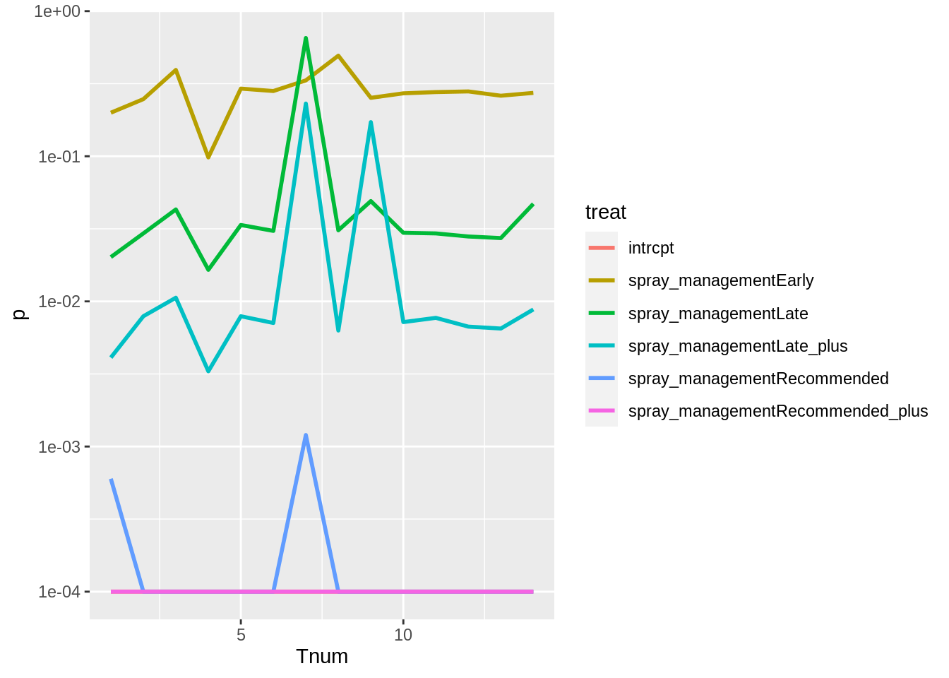

unique(PM_dat_D$trial_ref)[7]

## [1] "mung1617/02"

sensitiviy_df %>%
   group_by(treat) %>%
   summarise(
      minEst = min(estimates),
      medEst = median(estimates),
      maxEst = max(estimates),
      minP = min(p),
      medP = median(p),
      maxP = max(p)
   )

## # A tibble: 6 × 7
##   treat                            minEst medEst maxEst   minP    medP   maxP
##   <chr>                             <dbl>  <dbl>  <dbl>  <dbl>   <dbl>  <dbl>
## 1 intrcpt                            1.39  2.51   2.73  0.0001 0.0001  0.0001
## 2 spray_managementEarly             -1.08 -0.519 -0.412 0.0982 0.275   0.493 
## 3 spray_managementLate              -1.54 -1.26  -0.224 0.0165 0.0302  0.653 
## 4 spray_managementLate_plus         -1.83 -1.61  -0.500 0.0033 0.00745 0.231 
## 5 spray_managementRecommended       -2.32 -1.89  -1.06  0.0001 0.0001  0.0012
## 6 spray_managementRecommended_plus  -3.07 -2.58  -1.82  0.0001 0.0001  0.0001

While estimates and P values remained the mostly same when each trial was dropped from the analysis. Estimates changed the most when Trial 1617/02 at Missen Flats in 2017 was ommited from the analysis.

Calculation of I^2.

W <- diag(1 / (PM_dat_D$vi_logit + 0.0001))
X <- model.matrix(PMsev_mvPer)
P <- W - W %*% X %*% solve(t(X) %*% W %*% X) %*% t(X) %*% W
100 * sum(PMsev_mvPer$sigma2) / (sum(PMsev_mvPer$sigma2) + (PMsev_mvPer$k -
                                                               PMsev_mvPer$p) / sum(diag(P)))

## [1] 99.93606

100 * PMsev_mvPer$sigma2 / (sum(PMsev_mvPer$sigma2) + (PMsev_mvPer$k - PMsev_mvPer$p) /
                               sum(diag(P)))

## [1] 99.93606

This indicates that approximate amount of total variance attributed to trials/ clusters is 99%, which is very high. However given that many of the means included in the model contained an accompanying sample variance of zero, this might have been expected.

The estimates and significance from this model better reflect the distribution of raw values. In addition the residuals from this model are more evenly distributed. Let’s back transform the estimates.

backtransform <- function(m, input_only = FALSE, intercept) {
   if (input_only == FALSE) {
      intercept <- m$b[1]
      
      dat <- data.frame(
         estimates = inv_logit(c(intercept, m$b[-1] + intercept)),
         StdErr = inv_logit(m$se + intercept) - inv_logit(intercept),
         Zval = c(inv_logit(m$z[1]),
                  inv_logit(m$z[-1] + m$z[1]) - inv_logit(m$z[1])),
         Pval = reportP(m$pval, P_prefix = FALSE),
         CI_lb = c(inv_logit(m$ci.lb[1]),
                   inv_logit(m$ci.lb[-1] + intercept)),
         CI_ub = c(inv_logit(m$ci.ub[1]),
                   inv_logit(m$ci.ub[-1] + intercept)),
         row.names = colnames(m$G)
      )
   }
   if (input_only == TRUE) {
      if (missing(intercept))
         stop("'intercept' argument is empty")
      return(inv_logit(m + intercept) - inv_logit(intercept))
   }
   return(dat)
}

backtransform(PMsev_mvPer)

##                  estimates     StdErr        Zval     Pval     CI_lb     CI_ub
## control          0.9205527 0.02982578  0.99242160 < 0.0001 0.8122794 0.9687768
## Early            0.8772409 0.02870660 -0.01293451    0.313 0.7364486 0.9481188
## Late             0.7747212 0.03267812 -0.05399564   0.0315 0.5320236 0.9123010
## Late_plus        0.7104378 0.03329573 -0.09286533   0.0073 0.4410980 0.8840885
## Recommended      0.6480696 0.02613013 -0.35468527 < 0.0001 0.4437397 0.8095559
## Recommended_plus 0.4797860 0.02569827 -0.75652003 < 0.0001 0.2888949 0.6767677

5.1.1 Disease severity moderator contrasts

Calculate the treatment contrasts without back-transformation.

source("R/simple_summary.R") #function to provide a table that includes the treatment names in the contrasts

intercept <- PMsev_mvPer$b[1, 1]
z <- PMsev_mvPer$zval[1]

contrast_Ssum <-
   simple_summary(summary(glht(PMsev_mvPer, linfct = cbind(
      contrMat(rep(1, 6), type = "Tukey")
   )), test = adjusted("none")))

contrast_Ssum[6:15, ] %>%
   flextable() %>%
   autofit()

contrast	coefficients	StdErr	Zvalue	pvals	sig
Late - Early	-0.7314	0.6346	-1.1525	0.2491
Late_plus - Early	-1.0690	0.6475	-1.6510	0.0987
Recommended - Early	-1.3560	0.5373	-2.5236	0.0116	*
Recommended_plus - Early	-2.0475	0.5263	-3.8906	< 0.0001	***
Late_plus - Late	-0.3377	0.4608	-0.7328	0.4637
Recommended - Late	-0.6246	0.4244	-1.4718	0.1411
Recommended_plus - Late	-1.3161	0.4175	-3.1524	0.0016	**
Recommended - Late_plus	-0.2869	0.4171	-0.6880	0.4914
Recommended_plus - Late_plus	-0.9784	0.4131	-2.3682	0.0179	*
Recommended_plus - Recommended	-0.6915	0.2400	-2.8807	0.004	**

par(mar = c(5, 13, 4, 2) + 0.1)
plot(glht(PMsev_mvPer, linfct = cbind(contrMat(rep(
   1, 6
), type = "Tukey"))), yaxt = 'n')
axis(
   2,
   at = seq_along(contrast_Ssum$contrast),
   labels = rev(contrast_Ssum$contrast),
   las = 2,
   cex.axis = 0.8
)

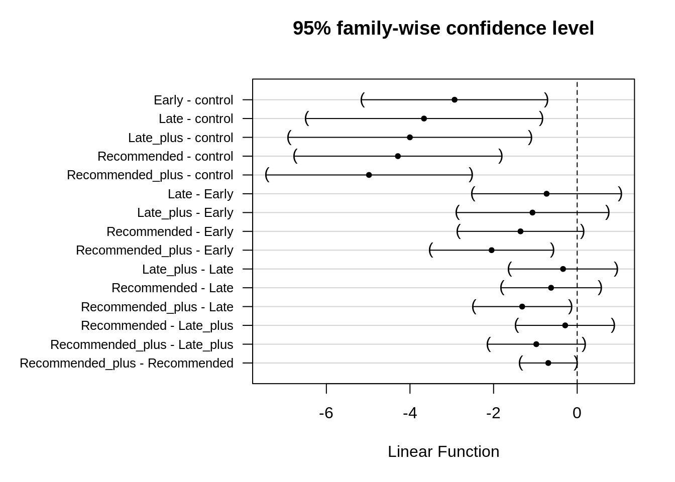
Recommended_plus limited disease severity significantly better than any other spray treatment. Early sprays were not effective in decreasing disease severity. Two spray treatments were significantly better than a single application, but the timing of the fungicide application was more critical.

5.1.2 Meta-analysis summary table

# obtain number of treatments included in each moderator variable
k5 <-
   as.data.frame(table(PM_dat_D$spray_management)) %>%
   filter(Freq != 0) %>%
   pull(Freq)

k6 <-
   as.data.frame(table(PM_dat_D$trial_ref, PM_dat_D$spray_management)) %>%
   filter(Freq != 0) %>%
   group_by(Var2) %>%
   summarise(n()) %>%
   pull()


# create data.frame of percent disease severity estimates
results_mv <- cbind(data.frame(
   Moderator = c(
      "Intercept / No Spray control",
      "Early",
      "Late",
      "Late+",
      "Recommended",
      "Recommended+"
   ),
   N = k5,
   k = k6
),
backtransform(PMsev_mvPer))

# Calculate mean differences
Intcpt <- results_mv$estimates[1]
results_mv <-
   results_mv %>%
   mutate(
      estimates = estimates - Intcpt,
      CI_lb = CI_lb - Intcpt,
      CI_ub = CI_lb - Intcpt
   )

# round the numbers
results_mv[, c(4:6, 8:9)] <- round(results_mv[, c(4:6, 8:9)], 4)

# rename colnames to give table headings
colnames(results_mv)[c(1:9)] <-
   c("Moderator",
     "N",
     "k",
     "mu",
     "se",
     "Z",
     "P",
     "CI_{L}",
     "CI_{U}")

disease_estimates_table <-
   results_mv[c(2, 5, 6, 3, 4), -6] %>%
   flextable() %>%
   align(j = 2:8, align = "center", part = "all") %>%
   fontsize(size = 8, part = "body") %>%
   fontsize(size = 10, part = "header") %>%
   italic(italic = TRUE, part = "header") %>%
   set_caption(
      "Table 3: Estimated powdery mildew severity mean difference for each spray schedule treatment to the unsprayed control treatments. Meta-analysis estimates were back transformed using an inverse logit. Data were obtained from the grey literature reports of (k) field trials undertaken in Eastern Australia. P values indicate statistical significance in comparison to the intercept."
   ) %>%
   footnote(
      i = 1,
      j = c(2:4, 6:8),
      value = as_paragraph(
         c(
            "Number of treatment means categorised to each spray schedule",
            "Number of trials with the respective spray schedule",
            "Estimated mean disease severity",
            "Indicates the significance between each respective spray schedule and the no spray control (intercept)",
            "Lower range of the 95% confidence interval",
            "Upper range of the 95% confidence interval"
         )
      ),
      ref_symbols = letters[c(1:6)],
      part = "header",
      inline = TRUE
   ) %>%
   hline_top(part = "all",
             border = officer::fp_border(color = "black", width = 2)) %>%
   width(j = 1, width = 1) %>%
   width(j = 2, width = 0.3) %>%
   width(j = 3, width = 0.3) %>%
   width(j = 4:8, width = 0.6)

disease_estimates_table

(#tab:metafor_results)Table 3: Estimated powdery mildew severity mean difference for each spray schedule treatment to the unsprayed control treatments. Meta-analysis estimates were back transformed using an inverse logit. Data were obtained from the grey literature reports of (k) field trials undertaken in Eastern Australia. P values indicate statistical significance in comparison to the intercept.
Moderator	Na	kb	muc	se	Pd	CI_{L}e	CI_{U}f
Early	13	3	-0.0433	0.0287	0.313	-0.1841	-1.1047
Recommended	28	12	-0.2725	0.0261	< 0.0001	-0.4768	-1.3974
Recommended+	41	11	-0.4408	0.0257	< 0.0001	-0.6317	-1.5522
Late	15	5	-0.1458	0.0327	0.0315	-0.3885	-1.3091
Late+	13	2	-0.2101	0.0333	0.0073	-0.4795	-1.4000
aNumber of treatment means categorised to each spray schedule; bNumber of trials with the respective spray schedule; cEstimated mean disease severity; dIndicates the significance between each respective spray schedule and the no spray control (intercept); eLower range of the 95% confidence interval; fUpper range of the 95% confidence interval

Kelly, Lisa, Jo White, Murray Sharman, Hugh Brier, Liz Williams, Raechelle Grams, Duncan Weir, Alan Mckay, and Adam H. Sparks. 2017. “Mungbean and sorghum disease update - GRDC.” https://grdc.com.au/resources-and-publications/grdc-update-papers/tab-content/grdc-update-papers/2017/07/mungbean-and-sorghum-disease-update.

Madden, L. V., H. P. Piepho, and P. A. Paul. 2016. “Statistical Models and Methods for Network Meta-Analysis.” Phytopathology 106 (8): 792–806. https://doi.org/10.1094/PHYTO-12-15-0342-RVW.

Thompson, Sue. 2016. “Mungbeans Vs Fungus: Two Sprays for Optimum Control - Grains Research and Development Corporation.” Ground Cover, September. https://grdc.com.au/resources-and-publications/groundcover/ground-cover-issue-124-septemberoctober-2016/mungbeans-vs-fungus-two-sprays-for-optimum-control.

Viechtbauer, Wolfgang. 2010. “Conducting Meta-Analyses in R with the metafor Package.” Journal of Statistical Software 36 (3): 1–48. https://doi.org/10.18637/jss.v036.i03.

4 Grain yield meta-analysis